Introduction
Overview
Teaching: 30 min
Exercises: 0 minQuestions
What will I learn during this workshop?
What are the tools that I will be using?
What are the tidy data principles?
What is working in a more open way beneficial?
Objectives
Discover a complete data analysis process revolving around the tidy principles.
Learn how to increase your data analysis efficacy
Table of contents
1. Overview
Welcome!
In this training you will learn R, RStudio, git, and GitHub. You will learn modern data science with R and the tidyverse suite of packages. It’s going to be fun and empowering! You will learn a reproducible workflow that can be used in research and analyses of all kinds.
In particular, you will learn about the concept of literate programming, a concept coined by Donald Kuth where a program code is made primarily to be read and understood by other people, and secondarily to be executed by the computer. This means that literate programs are very easy to understand and share, as all the code is well explained.
This training will get acquainted with these skills and best practices, you will get comfortable with a workflow that you can use in your own projects. Overall, you will
Three main takeaways
- Modern data transformation and visualization (R/RStudio,
tidyverse).- Collaborative version control (
git/GitHub).- Associating code and its description through literate programming (R Markdown/GitHub).
1.1 What to expect
This is going to be a fun workshop.
The plan is to expose you to a lot of great tools that you can have confidence using in your research. You’ll be working hands-on and doing the same things on your own computer as we do live on up on the screen. We’re going to go through a lot in these two days and it’s less important that you remember it all. More importantly, you’ll have experience with it and confidence that you can do it. The main thing to take away is that there are good ways to approach your analyses; we will teach you to expect that so you can find what you need and use it! A theme throughout is that tools exist and are being developed by real, and extraordinarily nice, people to meet you where you are and help you do what you need to do. If you expect and appreciate that, you will be more efficient in doing your awesome science.
You are all welcome here, please be respectful of one another. You are encouraged to help each other. We abide to the Carpentries Code of Conduct.
Everyone in this workshop is coming from a different place with different experiences and expectations. But everyone will learn something new here, because there is so much innovation in the data science world. Instructors and helpers learn something new every time, from each other and from your questions. If you are already familiar with some of this material, focus on how we teach, and how you might teach it to others. Use these workshop materials not only as a reference in the future but also for talking points so you can communicate the importance of these tools to your communities. A big part of this training is not only for you to learn these skills, but for you to also teach others and increase the value and practice of open data science in science as a whole.
1.2 What you will learn
- how to think about data
- how to think about data separately from your research questions.
- how and why to tidy data and analyze tidy data, rather than making your analyses accommodate messy data.
- how there is a lot of decision-making involved with data analysis, and a lot of creativity.
- how to increase efficiency in your data science
- foster reproducibility for you and others.
- facilitate collaboration with others — especially your future self!
- how Open Science is a great benefit
- Open Science is often good science: reproducible, clear, easy to share and access.
- broaden the impact of your work.
- ameliorate your scientific reputation.
- how to learn with intention and community
- think long-term instead of only to get a single job done now.
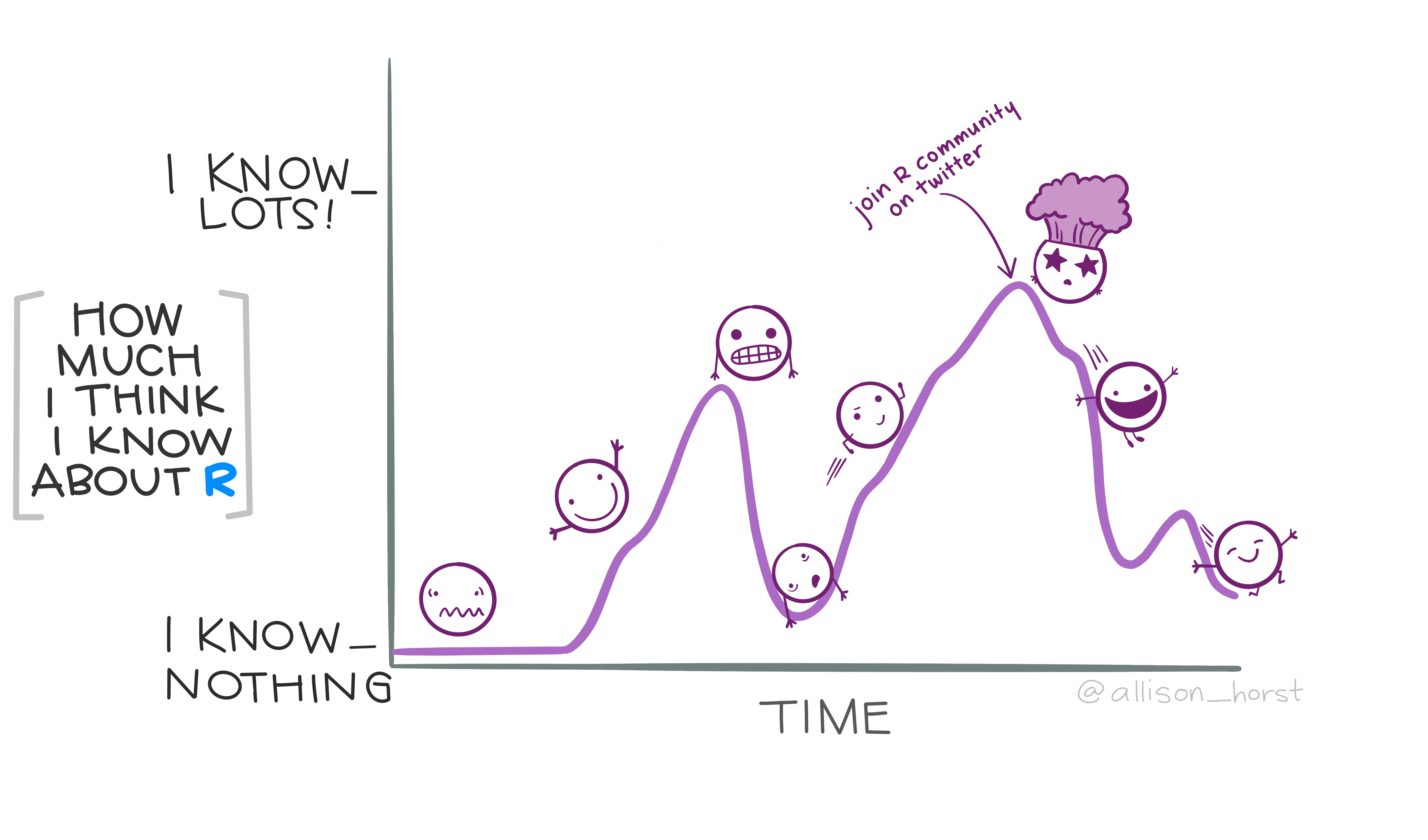
- the #rstats online community is fantastic. The tools we’re using are developed by real people. Real, nice people. They are building powerful and empowering tools and are welcoming to all skill-levels.
1.3 Be persistent
Learning a new programming language such as R and a new theme (data analysis) is not an easy task. Also, there is literally no end to learning, you will always find a better more smooth way to do things, a new package recently developed etc.
2. The tidy data workflow
We will be learning about tidy data. And how to use a tidyverse suite of tools to work with tidy data.
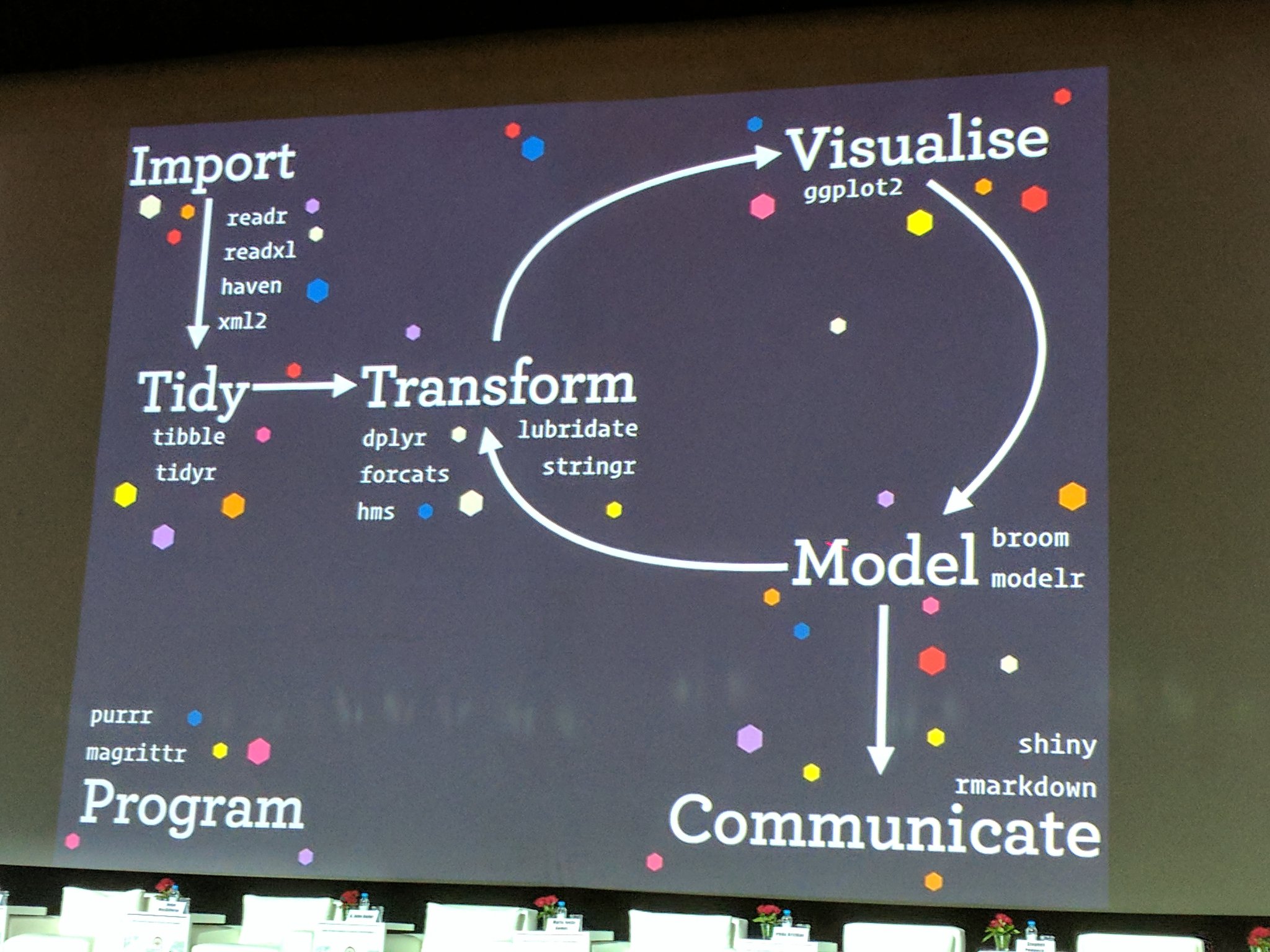
Hadley Wickham and his team have developed a ton of the tools we’ll use today. Here’s an overview of techniques to be covered in Hadley Wickham and Garrett Grolemund of RStudio’s book R for Data Science:
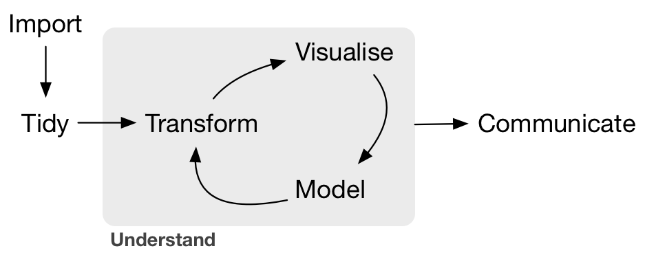
We will be focusing on:
- Tidy:
tidyrto organize rows of data into unique values. - Transform:
dplyrto manipulate/wrangle data based on subsetting by rows or columns, sorting and joining. - Visualize:
ggplot2static plots, using grammar of graphics principles. - Communicate: dynamic documents with
knitrto produce R Markdown notebooks.
This is really critical. Instead of building your analyses around whatever (likely weird) format your data are in, take deliberate steps to make your data tidy. When your data are tidy, you can use a growing assortment of powerful analytical and visualization tools instead of inventing home-grown ways to accommodate your data. This will save you time since you aren’t reinventing the wheel, and will make your work more clear and understandable to your collaborators (most importantly, Future You).
Reference: original paper about tidy datasets from Hadley Wickham.
2.1 Learning with public datasets
One of the most important things you will learn is how to think about data separately from your own research context. Said in another way, you’ll learn to distinguish your data questions from your research questions. Here, we are focusing on data questions, and we will use data that is not specific to your research.
We will be using several different data sets throughout this training, and will help you see the patterns and parallels to your own data, which will ultimately help you in your research.
2.2 Emphasizing collaboration
Collaborating efficiently has historically been really hard to do. It’s only been the last 20 years or so that we’ve moved beyond mailing things with the postal service. Being able to email and get feedback on files through track changes was a huge step forward, but it comes with a lot of bookkeeping and reproduciblity issues (did I do my analyses with thesis_final_final.xls or thesis_final_usethisone.xls?). But now, open tools make it much easier to collaborate.
Working with collaborators in mind is critical for reproducibility. And, your most important collaborator is your future self. This training will introduce best practices using open tools, so that collaboration will become second nature to you!
2.3 By the end of the course
By the end of the course, you’ll wrangle a few different data sets, and make your own graphics that you’ll publish on webpages you’ve built collaboratively with GitHub and RMarkdown. Woop!
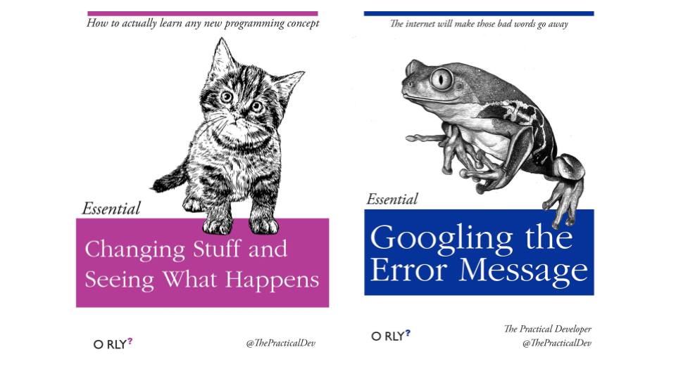
Here are some important things to keep in mind as you learn (these are joke book covers):
3. Credits
This lesson has been formatted according to the Carpentries Foundation lesson template and following their recommendations on how to teach researchers good practices in programming and data analysis.
This material builds from a lot of fantastic materials developed by others in the open data science community. Most of the content derives from the Ocean Health Index Data Science Training which are greatly acknowledge for the quality of their teaching materials.
It also pulls from the following resources, which are highly recommended for further learning and as resources later on. Specific lessons will also cite more resources.
- R for Data Science by Hadley Wickham and Garrett Grolemund
- STAT 545 by Jenny Bryan
- Happy Git with R by Jenny Bryan
- Software Carpentry by the Carpentries
- Artwork from @juliesquid for @openscapes (illustrated by @allison_horst).
- Artwort from @allisonhorst rstats illustrations
Key Points
Tidy data principles are essential to increase data analysis efficiency and code readability.
Using R and RStudio, it becomes easier to implement good practices in data analysis.
I can make my workflow more reproducible and collaborative by using git and Github.
R & RStudio, R Markdown
Overview
Teaching: 50 min
Exercises: 10 minQuestions
How do I orient myself in the RStudio interface?
How can I work with R in the console?
What are built-in R functions and how do I use their help page?
How can I generate an R Markdown notebook?
Objectives
Learn what is an Integrated Developing Environment.
Learn to work in the R console interactively.
Learn how to generate a reproducible code notebook with R Markdown.
Learn how to create an HTML or PDF document from a R Markdown notebook.
Understand that R Markdown notebooks foster literate programming, reproducibility and open science.
Table of Contents
- 1. Introduction
- 2. A quick touR
- 3. Diving deepeR
- 4. R Markdown notebook
- 5. Import your own data
- 6. Credits and additional resources
1. Introduction
This episode is focusing on the concept of literate programming supported by the ability to combine code, its output and human-readable descriptions in a single R Markdown document.
Literate programming
More generally, the mixture of code, documentation (conclusion, comments) and figures in a notebook is part of the so-called “literate programming” paradigm (Donald Knuth, 1984). Your code and logical steps should be understandable for human beings. In particular these four tips are related to this paradigm:
- Do not write your program only for R but think also of code readers (that includes you).
- Focus on the logic of your workflow. Describe it in plain language (e.g. English) to explain the steps and why you are doing them.
- Explain the “why” and not the “how”.
- Create a report from your analysis using a R Markdown notebook to wrap together the data + code + text.
1.1 The R Markdown format
Dr. Jenny Bryan’s lectures from STAT545 at R Studio Education
Leave your mark
R Markdown allows you to convert your complete analysis into a single report that is easy to share and that should recapitulate the logic of your code and related outputs.
A variety of output formats are supported:
- Word document
- Powerpoint
- HTML
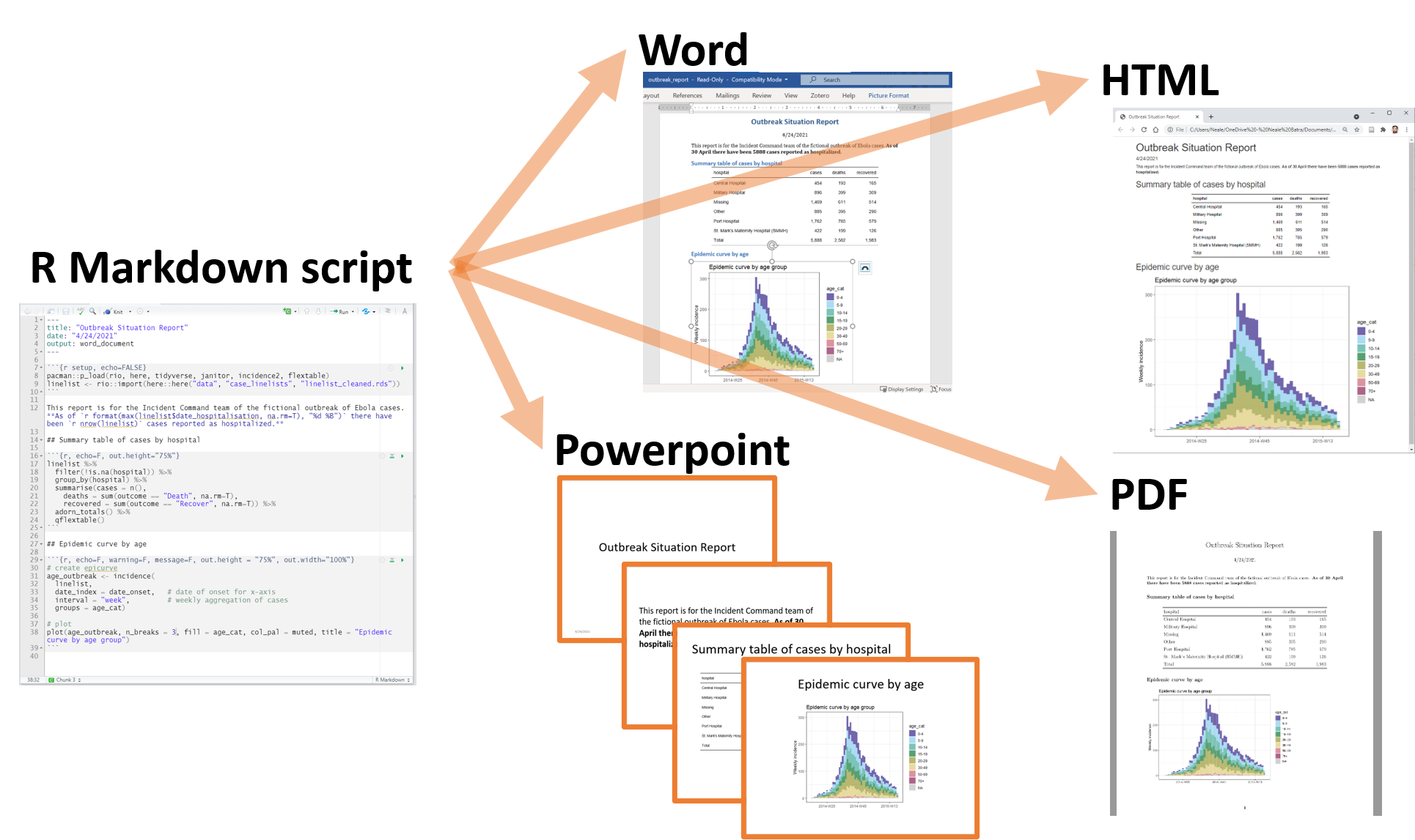
In practice, it is best practice to create a PDF document from your analysis as PDF documents are easy to open and visualise online especially on GitHub.
1.2 Why learn R with RStudio?
You are all here today to learn how to code. Coding made me a better scientist because I was able to think more clearly about analyses, and become more efficient in doing so. Data scientists are creating tools that make coding more intuitive for new coders like us, and there is a wealth of awesome instruction and resources available to learn more and get help.
Here is an analogy to start us off. Think of yourself as a pilot, and R is your airplane. You can use R to go places! With practice you’ll gain skills and confidence; you can fly further distances and get through tricky situations. You will become an awesome pilot and can fly your plane anywhere.
And if R were an airplane, RStudio is the airport. RStudio provides support! Runways, communication, community, and other services that makes your life as a pilot much easier. So it’s not only the infrastructure (the user interface or IDE), although it is a great way to learn and interact with your variables, files, and interact directly with GitHub. It’s also a data science philosophy, R packages, community, and more. So although you can fly your plane without an airport and we could learn R without RStudio, that’s not what we’re going to do.
Take-home message
We are learning R together with RStudio because it offers the power of a programming language with the comfort of an Integrated Development Environment.
Something else to start us off is to mention that you are learning a new language here. It’s an ongoing process, it takes time, you’ll make mistakes, it can be frustrating, but it will be overwhelmingly awesome in the long run. We all speak at least one language; it’s a similar process, really. And no matter how fluent you are, you’ll always be learning, you’ll be trying things in new contexts, learning words that mean the same as others, etc, just like everybody else. And just like any form of communication, there will be miscommunications that can be frustrating, but hands down we are all better off because of it.
While language is a familiar concept, programming languages are in a different context from spoken languages, but you will get to know this context with time. For example: you have a concept that there is a first meal of the day, and there is a name for that: in English it’s “breakfast”. So if you’re learning Spanish, you could expect there is a word for this concept of a first meal. (And you’d be right: ‘desayuno’). We will get you to expect that programming languages also have words (called functions in R) for concepts as well. You’ll soon expect that there is a way to order values numerically. Or alphabetically. Or search for patterns in text. Or calculate the median. Or reorganize columns to rows. Or subset exactly what you want. We will get you increase your expectations and learn to ask and find what you’re looking for.
2. A quick touR
2.1 RStudio panes
Like a medieval window, RStudio has several panes (sections that divide the entire window).

Launch RStudio/R and identify the different panes.
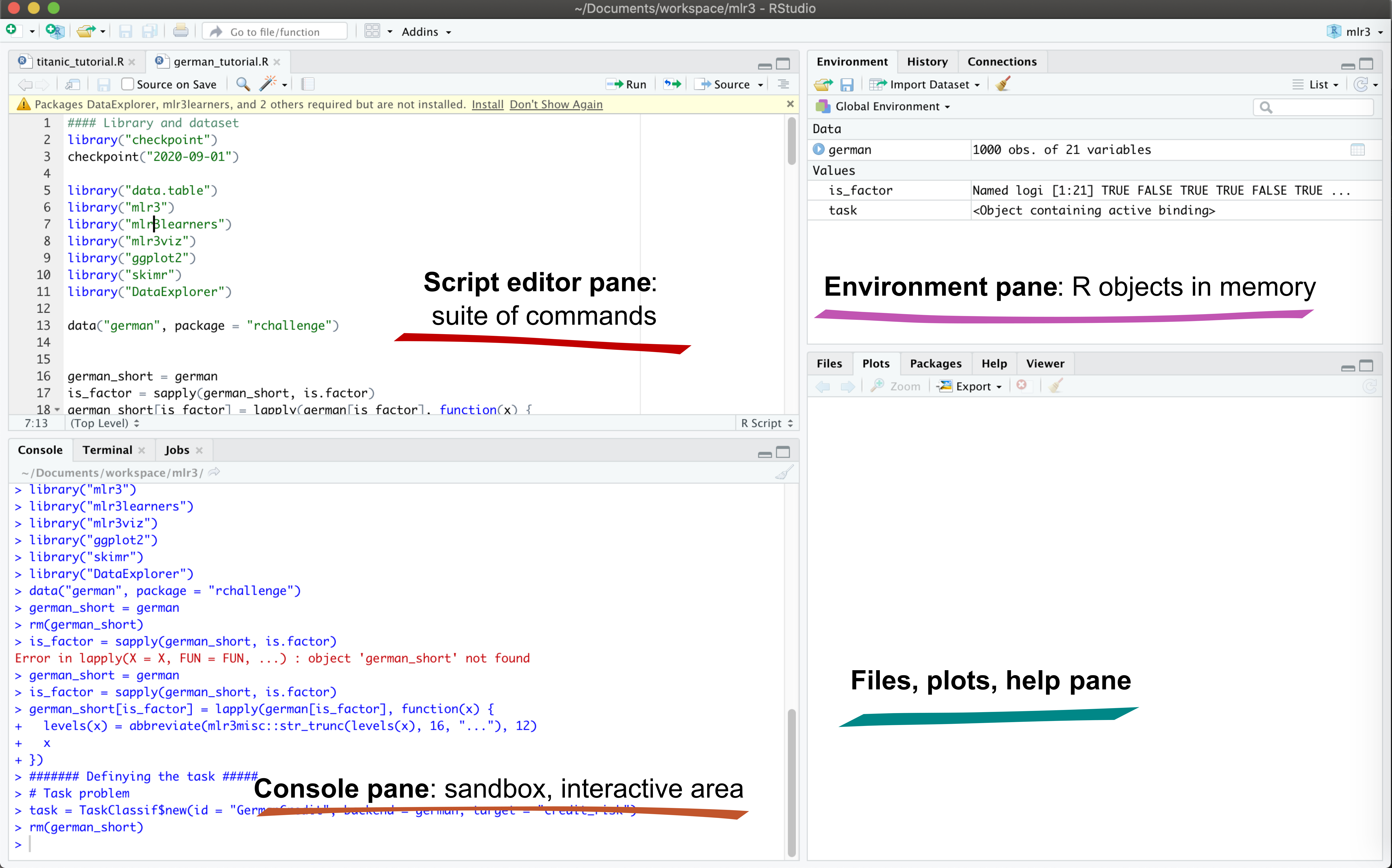
Notice the default panels:
- Script editor panel (upper left)
- Console (lower right)
- Environment/History (tabbed in upper right)
- Files/Plots/Packages/Help (tabbed in lower right)
Customizing RStudio appearance
You can change the default location of the panes, among many other things: Customizing RStudio.
2.2 Locating yourself
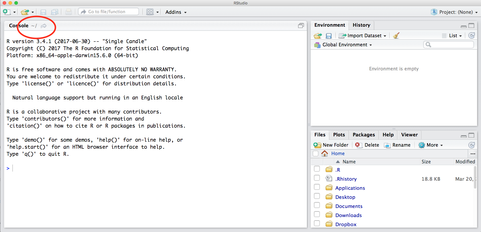
An important first question: where are we inside the computer file system?
If you’ve have opened RStudio for the first time, you’ll be in your home directory. This is noted by the ~/ at the top of the console. You can see too that the Files pane in the lower right shows what is in the home directory where you are. You can navigate around within that Files pane and explore, but note that you won’t change where you are: even as you click through you’ll still be Home: ~/.
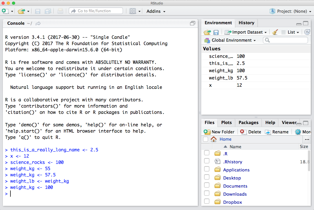
2.3 First step in the console
OK let’s go into the Console, where we interact with the live R process.
Make an assignment and then inspect the object you created by typing its name on its own.
x <- 3 * 4
x
In my head, I hear e.g., “x gets 12”.
All R statements where you create objects – “assignments” – have this form: objectName <- value.
I’ll write it in the console with a hashtag #, which is the way R comments so it won’t be evaluated.
## objectName <- value

## This is also how you write notes in your code to explain what you are doing.
Object names cannot start with a digit and cannot contain certain other characters such as a comma or a space. You will be wise to adopt a convention for demarcating words in names.
# i_use_snake_case
# other.people.use.periods
# evenOthersUseCamelCase
Make an assignment
this_is_a_really_long_name <- 2.5
To inspect this variable, instead of typing it, we can press the up arrow key and call your command history, with the most recent commands first. Let’s do that, and then delete the assignment:
this_is_a_really_long_name
Another way to inspect this variable is to begin typing this_…and RStudio will automagically have suggested completions for you that you can select by hitting the tab key, then press return.
One more:
science_rocks <- "yes it does!"
You can see that we can assign an object to be a word, not a number. In R, this is called a “string”, and R knows it’s a word and not a number because it has quotes " ". You can work with strings in your data in R pretty easily, thanks to the stringr and tidytext packages. We won’t talk about strings very much specifically, but know that R can handle text, and it can work with text and numbers together (this is a huge benefit of using R).
Let’s try to inspect:
sciencerocks
# Error: object 'sciencerocks' not found
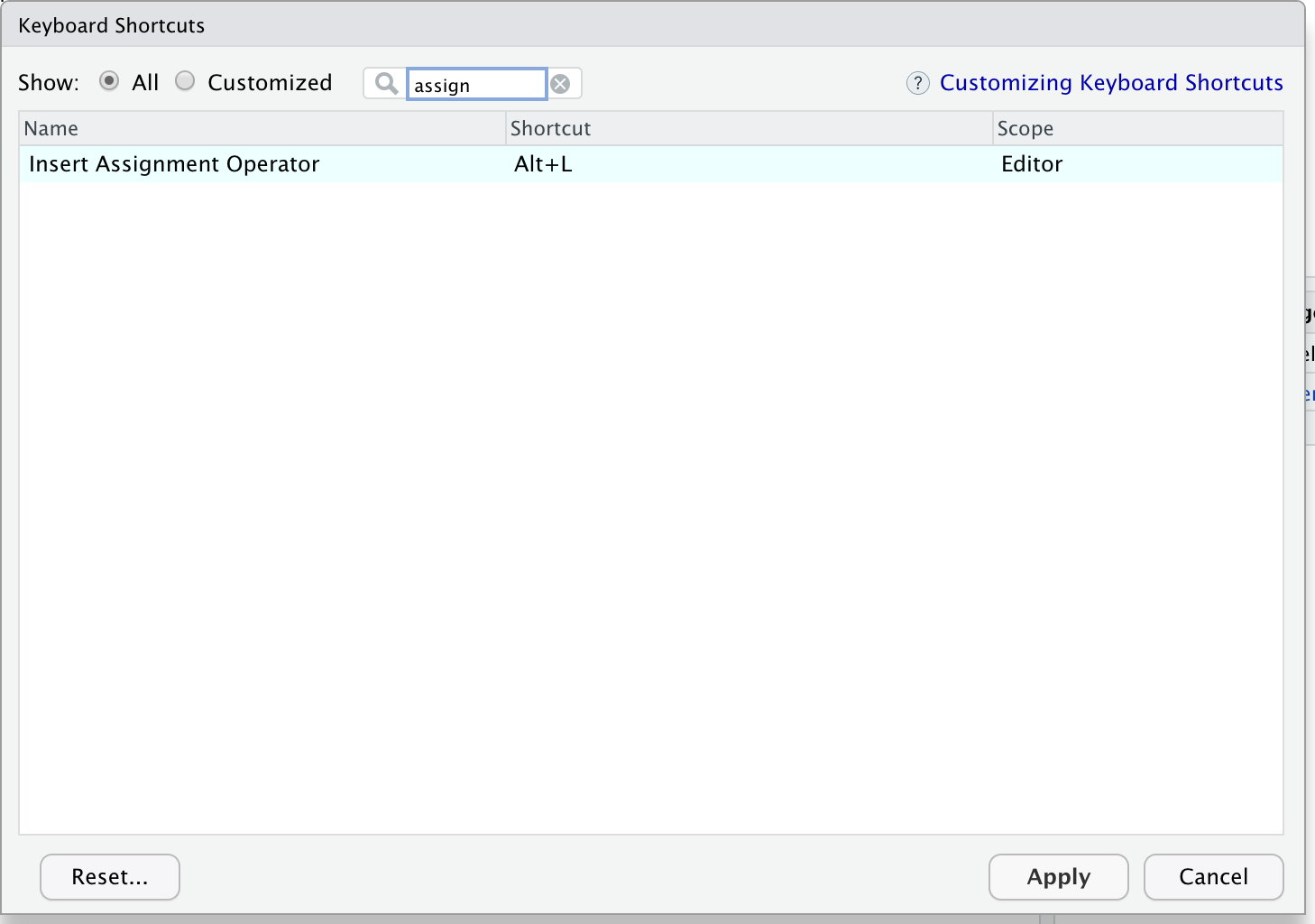
2.4 Make your life easier with keyboard shortcuts
One can rapidly experience that typing the assign operator <- is laborious to type in the long run. Instead, we can create a keyboard shortcut to make our life easier.
With RStudio, this is relatively straightforward. Follow the screenshots to change the default to Alt + L for instance.
Go to “Tools” followed by “Modify Keyboard Shortcuts”:
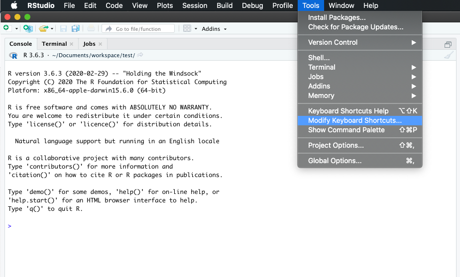
Then in the “Filter” text box, type “assign” to find the current keyboard shortcut for the assign operator. Change it to Alt + L or any other convenient key combination.
Lovely keyboard shortcuts:
RStudio offers many handy keyboard shortcuts.
Also,Alt + Shift + Kbrings up a keyboard shortcut reference card.
2.5 Error messages are your friends
Implicit contract with the computer / scripting language: Computer will do tedious computation for you. In return, you will be completely precise in your instructions. Typos matter. Case matters. Pay attention to how you type.
Remember that this is a language, not unsimilar to English! There are times you aren’t understood – it’s going to happen. There are different ways this can happen. Sometimes you’ll get an error. This is like someone saying ‘What?’ or ‘Pardon’? Error messages can also be more useful, like when they say ‘I didn’t understand what you said, I was expecting you to say blah’. That is a great type of error message. Error messages are your friend. Google them (copy-and-paste!) to figure out what they mean.
And also know that there are errors that can creep in more subtly, when you are giving information that is understood, but not in the way you meant. Like if I am telling a story about suspenders that my British friend hears but silently interprets in a very different way (true story). This can leave me thinking I’ve gotten something across that the listener (or R) might silently interpreted very differently. And as I continue telling my story you get more and more confused… Clear communication is critical when you code: write clean, well documented code and check your work as you go to minimize these circumstances!
2.6 Logical operators and expressions
A moment about logical operators and expressions. We can ask questions about the objects we made.
==means ‘is equal to’!=means ‘is not equal to’<means ‘is less than’>means ‘is greater than’<=means ‘is less than or equal to’>=means ‘is greater than or equal to’
x == 2
x <= 30
x != 5
2.7 Variable assignment
Let’s assign a number to a variable called weight_kg.
weight_kg <- 55    # doesn't print anything
(weight_kg <- 55)  # but putting parenthesis around the call prints the value of `weight_kg`
weight_kg          # and so does typing the name of the object
When assigning a value to an object, R does not print anything. You can force R to print the value by using parentheses or by typing the object name:
Now that R has weight_kg in memory, we can do arithmetic with it. For
instance, we may want to convert this weight into pounds (weight in pounds is 2.2 times the weight in kg):
weight_kg * 2.2
We can also change a variable’s value by assigning it a new one:
weight_kg <- 57.5
weight_kg * 2.2
And when we multiply it by 2.2, the outcome is based on the value currently assigned to the variable.
OK, let’s store the animal’s weight in pounds in a new variable, weight_lb:
weight_lb <- weight_kg * 2.2
and then change weight_kg to 100.
weight_kg <- 100
What do you think is the current content of the object weight_lb? 126.5 or 220? Why?
It’s 125.6. Why? Because assigning a value to one variable does not change the values of
other variables — if you want weight_kg updated to reflect the new value for weight_lb, you will have to re-execute that code. This is why we re-comment working in scripts and documents rather than the Console, and will introduce those concepts shortly and work there for the rest of the day.
We can create a vector of multiple values using c().
c(weight_lb, weight_kg)

names <- c("Jamie", "Melanie", "Julie")
names
Exercise
- Create a vector that contains the different weights of four fish (you pick the object name!):
- one fish: 12 kg
- two fish: 34 kg
- red fish: 20 kg
- blue fish: 6.6 kg
- Convert the vector of kilos to pounds (hint: 1 kg = 2.2 pounds).
- Calculate the total weight.
Solution
# Q1
fish_weights <- c(12, 34, 20, 6.6)
# Q2
fish_weights_lb <- fish_weights * 2.2
# Q3
# we haven't gone over functions like `sum()` yet but this is covered in the next section.
sum(fish_weights_lb)
3. Diving deepeR
3.1 Functions and help pages
R has a mind-blowing collection of built-in functions that are used with the same syntax: function name with parentheses around what the function needs to do what it is supposed to do.
function_name(argument1 = value1, argument2 = value2, ...). When you see this syntax, we say we are “calling the function”.
Let’s try using seq() which makes regular sequences of numbers and, while we’re at it, demo more helpful features of RStudio.
Type se and hit TAB. A pop up shows you possible completions. Specify seq() by typing more to disambiguate or using the up/down arrows to select. Notice the floating tool-tip-type help that pops up, reminding you of a function’s arguments. If you want even more help, press F1 as directed to get the full documentation in the help tab of the lower right pane.
Type the arguments 1, 10 and hit return.
seq(1, 10)
We could probably infer that the seq() function makes a sequence, but let’s learn for sure. Type (and you can autocomplete) and let’s explore the help page:
?seq
help(seq) # same as ?seq
Help page
The help page tells the name of the package in the top left, and broken down into sections:
- Description: An extended description of what the function does.
- Usage: The arguments of the function and their default values.
- Arguments: An explanation of the data each argument is expecting.
- Details: Any important details to be aware of.
- Value: The data the function returns.
- See Also: Any related functions you might find useful.
- Examples: Some examples for how to use the function.
seq(from = 1, to = 10) # same as seq(1, 10); R assumes by position
seq(from = 1, to = 10, by = 2)
The above also demonstrates something about how R resolves function arguments. You can always specify in name = value form. But if you do not, R attempts to resolve by position. So above, it is assumed that we want a sequence from = 1 that goes to = 10. Since we didn’t specify step size, the default value of by in the function definition is used, which ends up being 1 in this case. For functions I call often, I might use this resolve by position for the first
argument or maybe the first two. After that, I always use name = value.
The examples from the help pages can be copy-pasted into the console for you to understand what’s going on. Remember we were talking about expecting there to be a function for something you want to do? Let’s try it.
Exercise
Talk to your neighbor(s) and look up the help file for a function that you know or expect to exist. Here are some ideas:
?getwd()?plot()min()max()?mean()?log())Solution
- Gets and prints the current working directory.
- Plotting function.
- Minimum value in a vector or dataframe column.
- Maximum value in a vector or dataframe column.
- Geometric mean (average) of a vector or dataframe column. Generic function for the (trimmed) arithmetic mean.
- Logarithm function. Specific functions exist for log2 and log10 calculations.
And there’s also help for when you only sort of remember the function name: double-question mark:
??install
Not all functions have (or require) arguments:
date()
3.2 Packages
So far we’ve been using a couple functions from base R, such as seq() and date(). But, one of the amazing things about R is that a vast user community is always creating new functions and packages that expand R’s capabilities. In R, the fundamental unit of shareable code is the package. A package bundles together code, data, documentation, and tests, and is easy to share with others. They increase the power of R by improving existing base R functionalities, or by adding new ones.
The traditional place to download packages is from CRAN, the Comprehensive R Archive Network, which is where you downloaded R. You can also install packages from GitHub, which we’ll do tomorrow.
You don’t need to go to CRAN’s website to install packages, this can be accomplished within R using the command install.packages("package-name-in-quotes"). Let’s install a small, fun package praise. You need to use quotes around the package name.:
install.packages("praise")
Now we’ve installed the package, but we need to tell R that we are going to use the functions within the praise package. We do this by using the function library().
What’s the difference between a package and a library?
Sometimes there is a confusion between a package and a library, and you can find people calling “libraries” to packages.
Please don’t get confused: library() is the command used to load a package, and it refers to the place where the package is contained, usually a folder on your computer, while a package is the collection of functions bundled conveniently.
library(praise)
Now that we’ve loaded the praise package, we can use the single function in the package, praise(), which returns a randomized praise to make you feel better.
praise()
3.3 Clearing the environment
Now look at the objects in your environment (workspace) – in the upper right pane. The workspace is where user-defined objects accumulate.
You can also get a listing of these objects with a few different R commands:
objects()
ls()
If you want to remove the object named weight_kg, you can do this:
rm(weight_kg)
To remove everything:
rm(list = ls())
or click the broom 🧹 in RStudio Environment panel.
For reproducibility, it is critical that you delete your objects and restart your R session frequently. You don’t want your whole analysis to only work in whatever way you’ve been working right now — you need it to work next week, after you upgrade your operating system, etc. Restarting your R session will help you identify and account for anything you need for your analysis.
We will keep coming back to this theme but let’s restart our R session together: Go to the top menus: Session > Restart R.
Exercise
Clear your workspace and create a few new variables. Create a variable that is the mean of a sequence of 1-20.
- What’s a good name for your variable?
- Does it matter what your “by” argument is? Why?
Solution
- Any meaningful and relatively short name is good. As a suggestion
mean_seqcould work.- Yes it does. By default “by” is equal to 1 but it can be changed to any increment number.
4. R Markdown notebook
R Markdown will allow you to create your own workflow, save it and generate a high quality report that you can share. It supports collaboration and reproducibility of your work. This is really key for collaborative research, so we’re going to get started with it early and then use it for the rest of the day.
Literate programming
More generally, the mixture of code, documentation (conclusion, comments) and figures in a notebook is part of the so-called “literate programming” paradigm (Donald Knuth, 1984). Your code and logical steps should be understandable for human beings. In particular these four tips are related to this paradigm:
- Do not write your program only for R but think also of code readers (that includes you).
- Focus on the logic of your workflow. Describe it in plain language (e.g. English) to explain the steps and why you are doing them.
- Explain the “why” and not the “how”.
- Create a report from your analysis using a R Markdown notebook to wrap together the data + code + text.
4.1 R Markdown video (1-minute)
What is R Markdown? from RStudio, Inc. on Vimeo.
A minute long introduction to R Markdown
This is also going to introduce us to the fact that RStudio is a sophisticated text editor (among all the other awesome things). You can use it to keep your files and scripts organized within one place (the RStudio IDE) while getting support that you expect from text editors (check-spelling and color, to name a few).
An R Markdown file will allow us to weave markdown text with chunks of R code to be evaluated and output content like tables and plots.
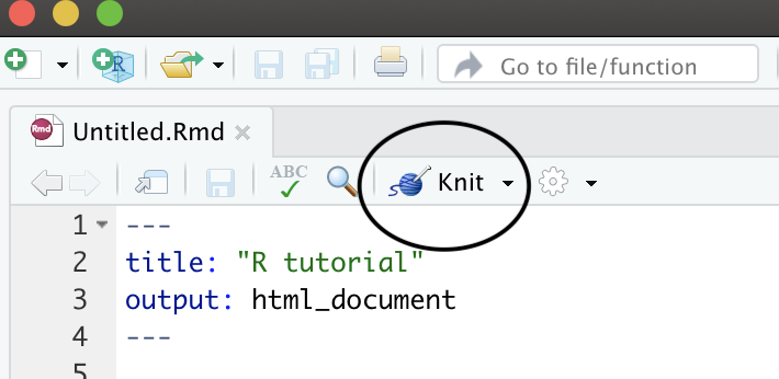
4.2 Create a R Markdown document
To do so, go to: File -> New File -> R Markdown… -> Document of output format HTML -> click OK.
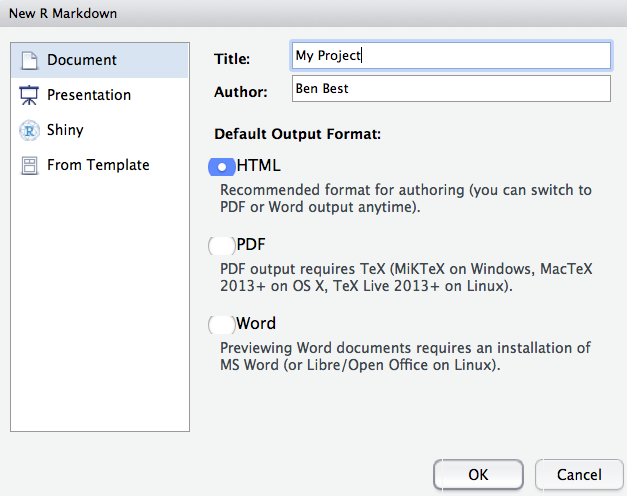
You can give it a Title like “R tutorial”. Then click OK.
Let’s have a look at this file — it’s not blank; there is some initial text is already provided for you. You can already notice a few parts:
- A document YAML header,
- Usually many different code chunks,
- and formatted text and various outputs (figures, tables)
4.3 The YAML header
The header of your R Markdown document will allow you to personalize the related report from your R Markdown document.
The header follows the YAML syntax (“YAML Ain’t Markup Language”) which usually follows a key:value syntax.
A few YAML parameters are all you need to know to start using R Markdown. Here is an opinionated list of the key parameters:
---
- title: "R tutorial"
- output: html_document
- author: "John Doe"
- date: "Tuesday, February 15 2021"
---
The three dashes --- before and after the option: value are important to delimit the YAML header. Do not forget them!
A note on output format: if you search online, you will find tons of potential output formats available from one R Markdown document. Some of them require additional packages or software installation. For instance, compiling your document to produce a PDF will require LaTeX libraries etc.
Exercise
Open the output formats of the R Markdown definitive guide: https://bookdown.org/yihui/rmarkdown/output-formats.html.
Instead ofoutput: html_document, specifypdf_documentto compile into a PDF (because it is easier to share for instance).
Press the knit button. Is it working? If not, what is missing?
For PDF, you might need to install a distribution of LaTeX for which several options exist. The recommended one is to install TinyTeX from Yihui Xie. Other more comprehensive LaTeX distributions can be obtained from the LaTeX project directly for your OS.
If you feel adventurous, you can try other formats. There are many things you can generate from a R Markdown document even slides for a presentation.
Exercise
Instead of hard-coding the date in the YAML section, search online for a way to dynamically have the today’s date.
Solution
In the YAML header, write:
date: r Sys.Date()
This will add today’s date in the YYYY-MM-DD format when compiling.
More generally, you can use the syntax option: r <some R command> to have options automatically updated by some R command when
compiling your R Markdown notebook into a report.
4.4 Code chunks
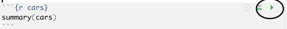
Code chunks appear in grey and will execute the R code when you compile the document.
The following chunk will create a summary of the cars dataframe.

A code chunk is defined by three backticks ```{r} before curly braces with r inside to indicate the coding language.
It is closed by three backticks ```.
```{r}
summary(cars)
```
The code chunk will be executed when compiling the report. You can also run it by clicking on the green arrow.
To insert a new code chunk, you can either:
- Use a keyboard shortcut:
Ctrl + Alt + I: to add a code chunk. UseCmd + Alt + Ion Mac OS. - Click on “Add chunk in the toolbar. “
- Place two code chunk:
```{r}to open the code chunk and```to close it.
Exercise
Introduce a new code chunk to produce a histogram of the cars speed.
Compile your R Markdown document and visualise the results.
In the final document, can you find a way to hide the code chunk that generates the plot?Solution
Add a new code chunk:
```{r}
hist(cars$speed)
```
Inside the curly braces, add:
```{r, echo = FALSE}
hist(cars$speed)
```
4.5 Text markdown syntax
You might wonder what the “markdown” in R Markdown stands for.
Between code chunks, you can write normal plain text to comment figures and code outputs. To format titles, paragraphs, format text in italics, etc. you can make use of the markdown syntax that is a simple but efficient method to format text. Altogether, it means that a R Markdown document has 2 different languages within it: R and Markdown.
Markdown is a formatting language for plain text, and there are only about 15 rules to know.
Have a look at your own document. Notice the syntax for:
- headers get rendered at multiple levels:
#,## - bold:
**word** - Web links:
<http://rmarkdown.rstudio.com>or[http://rmarkdown.rstudio.com](http://rmarkdown.rstudio.com).. - In line code: see the
echo = FALSE
There are some good cheatsheets to get you started, and here is one built into RStudio: Go to Help > Markdown Quick Reference
Exercise
In Markdown:
- Format text in italics,
- Make a numbered list,
- Add a web link to the RStudio website in your document,
- Add a “this is a subheader” subheader with the level 2 or 3.
Reknit your document.Solution
- Add one asterisk or one underscore on both sides of the text.
- To make a numbered list, write
1.then add a line and write a second2..- Place the link between squared brackets. RStudio link
- Subheaders can be written with
###or##depending on the level that you want to write.
A complete but short guide on Markdown syntax from Yihui Xie is available here.
4.6 Compile your R Markdown document
Now that we are all set, we can compile the document to generate the corresponding HTML document. Press the “Knit” button.
This will compile your R Markdown document and open a new window.
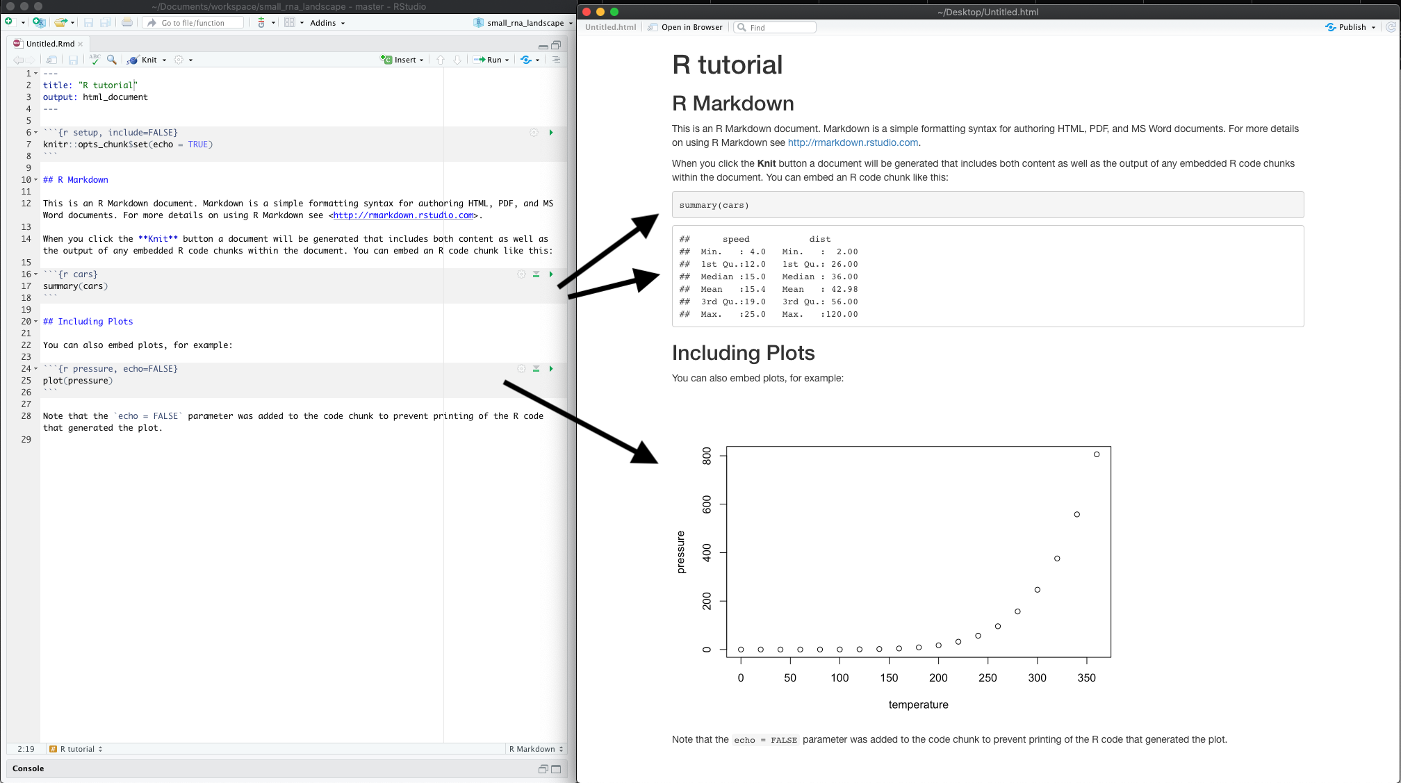
What do you notice between the two? So much of learning to code is looking for patterns.
Notice how the grey R code chunks are surrounded by 3 backticks and {r LABEL}. These are evaluated and return the output text in the case of summary(cars) and the output plot in the case of plot(pressure).
Notice how the code plot(pressure) is not shown in the HTML output because of the R code chunk option echo=FALSE.
Compiling takes place in a separate R workspace
When compiling, you will be redirected to the R Markdown tab next to your Console. This is normal as your R Markdown document is compiled in a separate new R workspace.
4.7 Useful tips and common issues
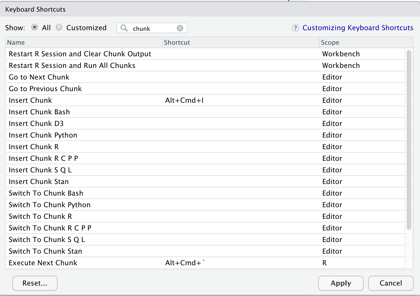
Here is a list of useful keyboard shortcuts:
Useful shortcuts
Place the cursor in the script editor pane. Then type:
Ctrl + Alt + I: to add a code chunk.Ctrl + Shift + K: compile the R Markdown document to create the related output.Ctrl + Alt + Cto run the current code chunk (your cursor has to be inside a code chunk).Ctrl + Alt + RFor Mac OS users, replace
CtrlwithCmd(Command).
All these shortcuts can be seen in Code > Run Region > …
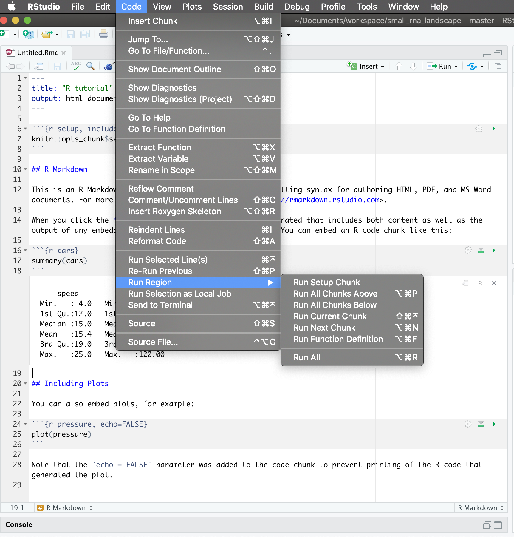
As seen before, you can modify these shortcuts to anything you find convenient: Tools > Modify keyboard shortcuts.
Type “chunk” to filter the shortcuts for code chunks.
Common issues
Separate workspace when compiling When you compile your R Markdown document, it will start from a clean R workspace. Anything you have in your current R interactive session will not be available in the R Markdown tab.
This is often the source of bugs and halting
Exercise
Step 1: In the R console, type:
library(dplyr)
tooth_filtered <- dplyr::filter(ToothGrowth, len > 1)
You should see the
tooth_filteredR object in your current environment.Step 2: in your R Markdown document, add this line:
with(tooth_filtered, hist(x = len, col = "darkgrey"))Try to knit your document. What bug do you experience?
Solution
Since your R Markdown workspace starts from scratch and creates a new environment, it ignores the
tooth_filteredobject you created in your R console.
The solution is to add thetooth_filtered <- dplyr::filter(ToothGrowth, len > 1)line inside a code chunk.
5. Import your own data
5.1 Functions available
To import your own data, you can use different functions depending on your input format:
read.tableis the generic function to import from various format. You do have to specify the separator as it is not known by default (tabulation or comma for instance).read.csvto import a table with comma-separated values (my_file.csv). You don’t have to specify the separator as it is by default a comma.read.delimto import a table with tabulated-separated values (my_file.tsvormy_file.txt). You don’t have to specify the separator as it is by default a tabulation.
Some important parameters in data import functions:
stringsAsFactors = TRUEis by default converting your characters into factors. This can be an issue for plotting for instance. I recommend to turn it off (stringsAsFactors = FALSEand change your strings to factors explicitely later on usingfactor()for instance.check.names = TRUEis by default checking your column names. For instance, if your column names start with a number, then R will prepend anXbefore your column variable name. To avoid this, addcheck.names = FALSE.
5.2 Important tips
Taken from Anna Krystalli workshop:
read.csv
read.csv(file,
	     na.strings = c("NA", "-999"),
         strip.white = TRUE,
         blank.lines.skip = TRUE,
         fileEncoding = "mac")
na.string: character vector of values to be coded missing and replaced with NA to argument egstrip.white: Logical. if TRUE strips leading and trailing white space from unquoted character fieldsblank.lines.skip: Logical: if TRUE blank lines in the input are ignored.fileEncoding: if you’re getting funny characters, you probably need to specify the correct encoding.
5.2 Large tables
If you have very large tables (1000s of rows and/or columns), use the fread() function from the data.table package.
6. Credits and additional resources
6.1 Jenny Bryan
- Stat 545 University module: https://stat545.com/
- Main website: https://jennybryan.org/
6.2 RStudio materials
- The official RStudio R Markdown documentation: https://rmarkdown.rstudio.com/
- The RStudio R Markdown cheatsheet
6.3 The definitive R Markdown guide
“The R Markdown definitive guide” by Yihui Xie, J. J. Allaire and Garrett Grolemund: https://bookdown.org/yihui/rmarkdown/
6.4 Others
- Remedy: additional functionalities for markdown in RStudio: https://thinkr-open.github.io/remedy/
- R Markdown Crash Course: a very complete course on R Markdown. https://zsmith27.github.io/rmarkdown_crash-course/
Key Points
R and RStudio make a powerful duo to create R scripts and R Markdown notebooks.
RStudio offers a text editor, a console and some extra features (environment, files, etc.).
R is a functional programming language: everything resolves around functions.
R Markdown notebook support code execution, report creation and reproducibility of your work.
Literate programming is a paradigm to combine code and text so that it remains understandable to humans, not only to machines.
Visualizing data with ggplot2
Overview
Teaching: 30 min
Exercises: 60 minQuestions
How can I make publication-grade plots with
ggplot2?What are the key concepts underlying
ggplot2plotting?What are some of the visualisations available through
ggplot2?How can I save my plot in a specific format (e.g. png)?
Objectives
Install the
ggplot2package by installing tidyverse.Learn basics of
ggplot2with several public datasets.Learn how to customize your plot efficiently (facets, geoms).
See how to use the stat functions to produce on-the-fly summary plots.
Table of Contents
- 1. Introduction
- 2. First plot with
ggplot2 - 3. Building your plots iteratively
- 4. Bar charts
- 5. Resources
1. Introduction
Why do we start with data visualization? Not only is data visualisation a big part of analysis, it’s a way to see your progress as you learn to code.
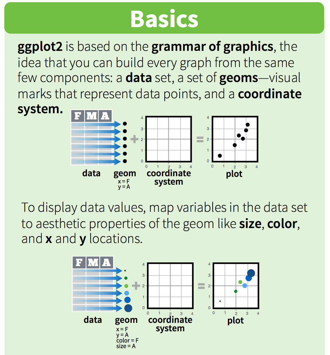
ggplot2implements the grammar of graphics, a coherent system for describing and building graphs. Withggplot2, you can do more faster by learning one system and applying it in many places. - Hadley Wickham, R for Data Science
This lesson borrows heavily from Hadley Wickham’s R for Data Science book, and an EcoDataScience lesson on Data Visualization.
1.1 Install our first package: tidyverse
Packages are bundles of functions, along with help pages and other goodies that make them easier for others to use, (ie. vignettes).
So far we’ve been using packages that are already included in base R. These can be considered out-of-the-box packages and include things such as sum and mean. You can also download and install packages created by the vast and growing R user community. The most traditional place to download packages is from CRAN, the Comprehensive R Archive Network. This is where you went to download R originally, and will go again to look for updates. You can also install packages directly from GitHub, which we’ll do tomorrow.
You don’t need to go to CRAN’s website to install packages, we can do it from within R with the command install.packages("package-name-in-quotes").
We are going to be using the package ggplot2, which is actually bundled into a huge package called tidyverse. We will install tidyverse now, and use a few functions from the packages within. Also, check out tidyverse.org/.
## from CRAN:
install.packages("tidyverse") ## do this once only to install the package on your computer.
library(tidyverse) ## do this every time you restart R and need it
When you do this, it will tell you which packages are inside of tidyverse that have also been installed. Note that there are a few name conflicts; it is alerting you that we’ll be using two functions from dplyr instead of the built-in stats package.
What’s the difference between install.packages() and library()? Why do you need both? Here’s an analogy:
install.packages()is setting up electricity for your house. Just need to do this once (let’s ignore monthly bills).library()is turning on the lights. You only turn them on when you need them, otherwise it wouldn’t be efficient. And when you quit R, it turns the lights off, but the electricity lines are still there. So when you come back, you’ll have to turn them on again withlibrary(), but you already have your electricity set up.
You can also install packages by going to the Packages tab in the bottom right pane. You can see the packages that you have installed (listed) and loaded (checkbox). You can also install packages using the install button, or check to see if any of your installed packages have updates available (update button). You can also click on the name of the package to see all the functions inside it — this is a super helpful feature that I use all the time.
1.2 Load national park datasets
Copy and paste the code chunk below and read it in to your RStudio to load the five datasets we will use in this section.
Important note
The
read_csv()function comes from thereadrpackage part of thetidyversesuite of packages. Make sure you’ve runlibrary(tidyverse)to load the datasets.
# National Parks in California
ca <- read_csv("https://raw.githubusercontent.com/carpentries-incubator/open-science-with-r/gh-pages/data/ca.csv")

# Acadia National Park
acadia <- read_csv("https://raw.githubusercontent.com/carpentries-incubator/open-science-with-r/gh-pages/data/acadia.csv")

# Southeast US National Parks
se <- read_csv("https://raw.githubusercontent.com/carpentries-incubator/open-science-with-r/gh-pages/data/se.csv")

# 2016 Visitation for all Pacific West National Parks
visit_16 <- read_csv("https://raw.githubusercontent.com/carpentries-incubator/open-science-with-r/gh-pages/data/visit_16.csv")

# All Nationally designated sites in Massachusetts
mass <- read_csv("https://raw.githubusercontent.com/carpentries-incubator/open-science-with-r/gh-pages/data/mass.csv")
2. First plot with ggplot2
ggplot2 is a plotting package that makes it simple to create complex plots from data in a data frame. It provides a more programmatic interface for specifying what variables to plot, how they are displayed, and general visual properties. Therefore, we only need minimal changes if the underlying data change or if we decide to change from a bar plot to a scatterplot. This helps in creating publication quality plots with minimal amounts of adjustments and tweaking.
ggplot likes data in the tidy (‘long’) format: i.e., a column for every dimension, and a row for every observation. Well structured data will save you lots of time when making figures with ggplot. We’ll learn more about tidy data in the next section.
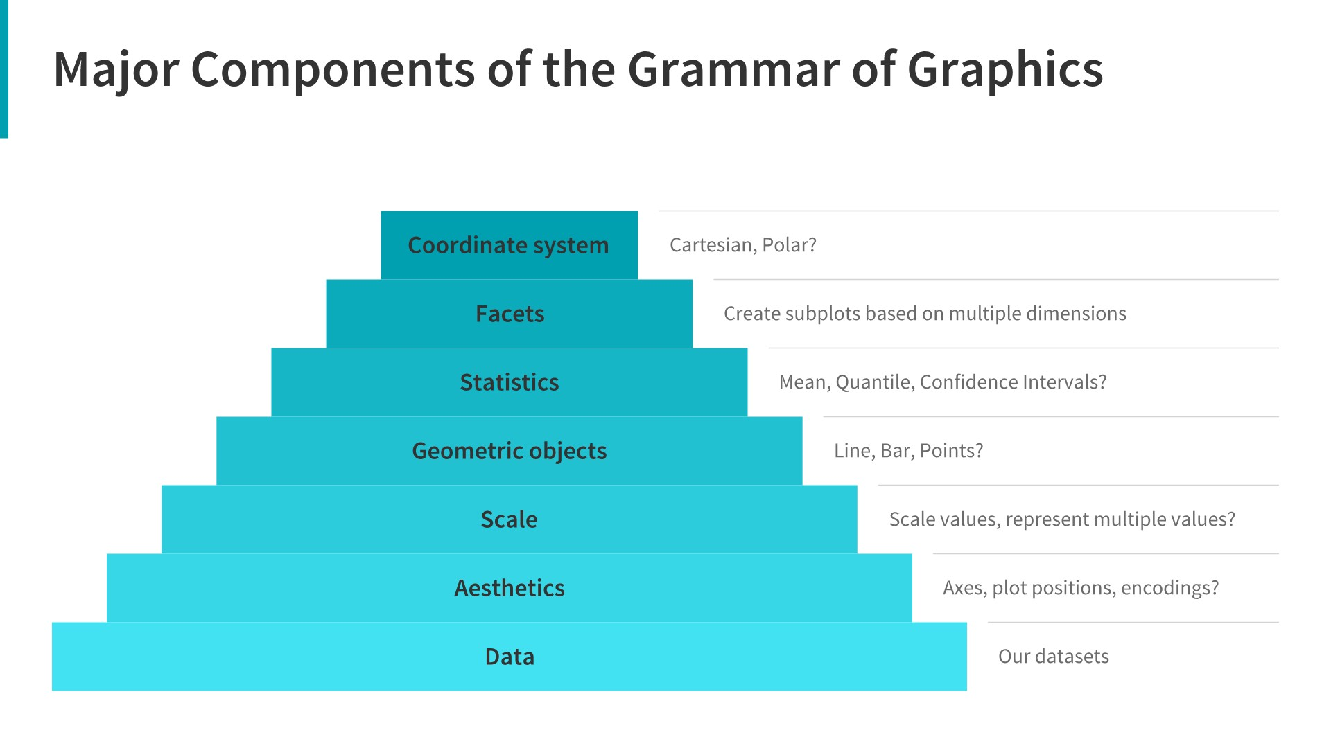
ggplot graphics are built step by step by adding new elements. Adding layers in this fashion allows for extensive flexibility and customization of plots.
One can see it as a pyramid of layers too.
2.1 Data description
We are going to use a National Park visitation dataset (from the National Park Service at https://irma.nps.gov/Stats/SSRSReports). Read in the data using read_csv and take a look at the first few rows using head() or View().
head(ca)
This dataframe is already in a tidy format where all rows are an observation and all columns are variables. Among the variables in ca are:
-
region, US region where park is located. -
visitors, the annual visitation for eachyear
# A tibble: 789 x 7
   region state code  park_name                     type          visitors  year
   <chr>  <chr> <chr> <chr>                         <chr>            <dbl> <dbl>
 1 PW     CA    CHIS  Channel Islands National Park National Park     1200  1963
 2 PW     CA    CHIS  Channel Islands National Park National Park     1500  1964
 3 PW     CA    CHIS  Channel Islands National Park National Park     1600  1965
 4 PW     CA    CHIS  Channel Islands National Park National Park      300  1966
 5 PW     CA    CHIS  Channel Islands National Park National Park    15700  1967
 6 PW     CA    CHIS  Channel Islands National Park National Park    31000  1968
 7 PW     CA    CHIS  Channel Islands National Park National Park    33100  1969
 8 PW     CA    CHIS  Channel Islands National Park National Park    32000  1970
 9 PW     CA    CHIS  Channel Islands National Park National Park    24400  1971
10 PW     CA    CHIS  Channel Islands National Park National Park    31947  1972
# … with 779 more rows
2.2 Building a plot
To build a ggplot, we need to:
- use the
ggplot()function and bind the plot to a specific data frame using thedataargument.
# initiate the plot
ggplot(data=ca)
- add
geoms– graphical representation of the data in the plot (points, lines, bars).ggplot2offers many different geoms; we will use some common ones today, including:
*geom_point()for scatter plots, dot plots, etc.
*geom_bar()for bar charts
*geom_line()for trend lines, time-series, etc.
To add a geom to the plot use + operator. Because we have two continuous variables, let’s use geom_point() first and then assign x and y aesthetics (aes).
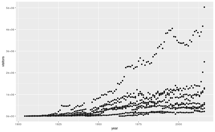
# add geoms
ggplot(data=ca) +
  geom_point(aes(x = year,y = visitors))
Notes:
- Anything you put in the
ggplot()function can be seen by any geom layers that you add (i.e., these are universal plot settings). This includes the x and y axis you set up inaes(). - You can also specify aesthetics for a given geom independently of the
aesthetics defined globally in the
ggplot()function. - The
+sign used to add layers must be placed at the end of each line containing a layer. If, instead, the+sign is added in the line before the other layer,ggplot2will not add the new layer and will return an error message.
3. Building your plots iteratively
Building plots with ggplot is typically an iterative process. We start by defining the dataset we’ll use, lay the axes, and choose a geom:
ggplot(data = ca) +
    geom_point(aes(x = year, y = visitors))
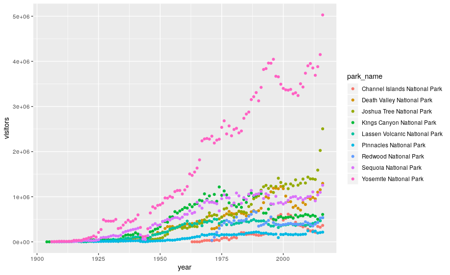
This isn’t necessarily a useful way to look at the data. We can distinguish each park by added the color argument to the aes:
ggplot(data=ca) +
  geom_point(aes(x = year, y = visitors, color = park_name))
3.1 Customizing plots
Take a look at the ggplot2 cheat sheet, and think of ways you could improve the plot.
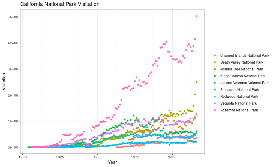
Now, let’s capitalize the x and y axis labels and add a main title to the figure. I also like to remove that standard gray background using a different theme. Many themes come built into the ggplot2 package. My preference is theme_bw() but once you start typing theme_ a list of options will pop up. The last thing I’m going to do is remove the legend title.
ggplot(data = ca) +
    geom_point(aes(x = year, y = visitors, color = park_name)) +
    labs(x = "Year",
       y = "Visitation",
       title = "California National Park Visitation") +
    theme_bw() +
    theme(legend.title=element_blank())
3.2 ggplot2 themes
In addition to theme_bw(), which changes the plot background to white, ggplot2 comes with several other themes which can be useful to quickly change the look of your visualization.
The ggthemes package provides a wide variety of options (including an Excel 2003 theme). The ggplot2 extensions website provides a list of packages that extend the capabilities of ggplot2, including additional themes.
Exercise
- Using the
sedataset, make a scatterplot showing visitation to all national parks in the Southeast region with color identifying individual parks.- Change the plot so that color indicates
state. Customize by adding your own title and theme. You can also change the text sizes and angles. Try applying a 45 degree angle to the x-axis. Use your cheatsheet!- In the following code, why isn’t the data showing up?
ggplot(data = se, aes(x = year, y = visitors))Solution
ggplot(data = se) + geom_point(aes(x = year, y = visitors, color = park_name)).- See the code below:
ggplot(data = se) +
 geom_point(aes(x = year, y = visitors, color = state)) +
labs(x = "Year", y = "Visitation", title = "Southeast States National Park Visitation") +theme_light() + theme(legend.title = element_blank(), axis.text.x = element_text(angle = 45, hjust = 1, size = 14))- The code is missing a geom to describe how the data should be plotted.
3.3 Faceting
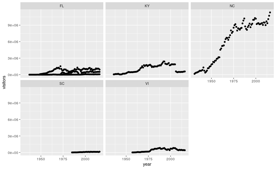
ggplot has a special technique called faceting that allows the user to split one plot into multiple plots based on data in the dataset. We will use it to make a plot of park visitation by state:
ggplot(data = se) +
    geom_point(aes(x = year, y = visitors)) +
    facet_wrap(~ state)
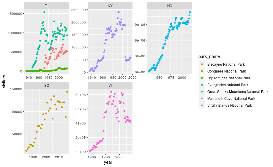
We can now make the faceted plot by splitting further by park using park_name (within a single plot):
 ggplot(data = se) +
     geom_point(aes(x = year, y = visitors, color = park_name)) +
     facet_wrap(~ state, scales = "free")
3.4 Geometric objects (geoms)
A geom is the geometrical object that a plot uses to represent data. People often describe plots by the type of geom that the plot uses. For example, bar charts use bar geoms, line charts use line geoms, boxplots use boxplot geoms, and so on.
Scatterplots break the trend; they use the point geom. You can use different geoms to plot the same data. To change the geom in your plot, change the geom function that you add to ggplot(). Let’s look at a few ways of viewing the distribution of annual visitation (visitors) for each park (park_name).
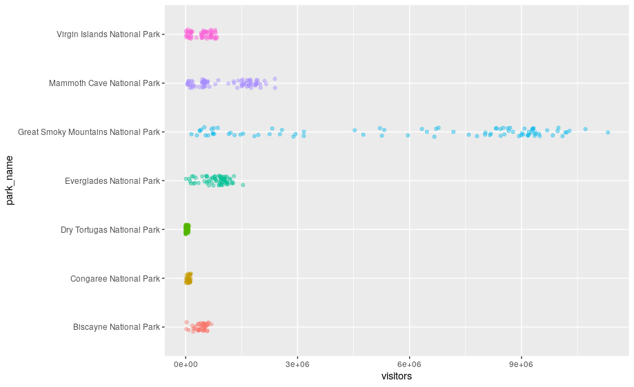
# representations as points with a jitter offset
ggplot(data = se) +
  geom_jitter(aes(x = park_name, y = visitors, color = park_name),
              width = 0.1,
              alpha = 0.4) +
  coord_flip() +
  theme(legend.position = "none")
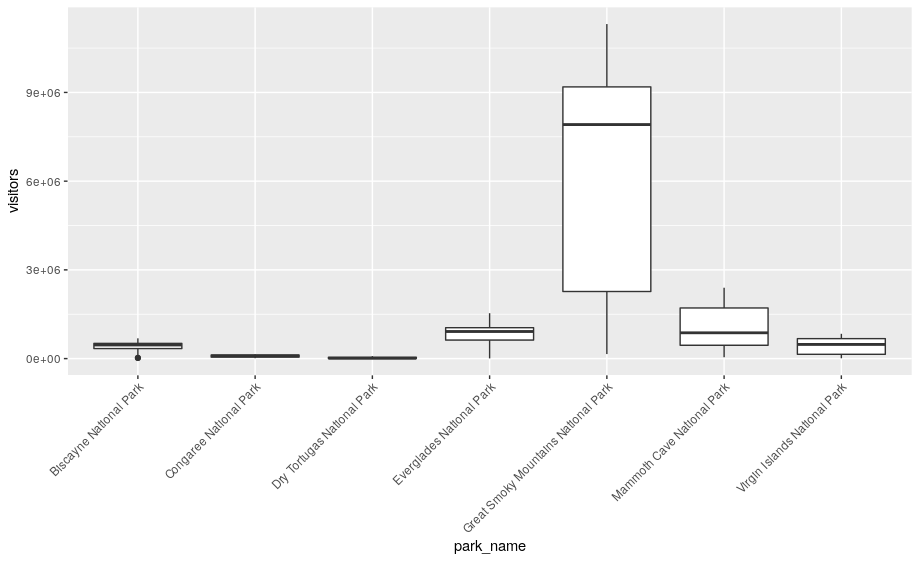
# boxplots
ggplot(se, aes(x = park_name, y = visitors)) +
  geom_boxplot() +
  theme(axis.text.x = element_text(angle = 45, hjust = 1))
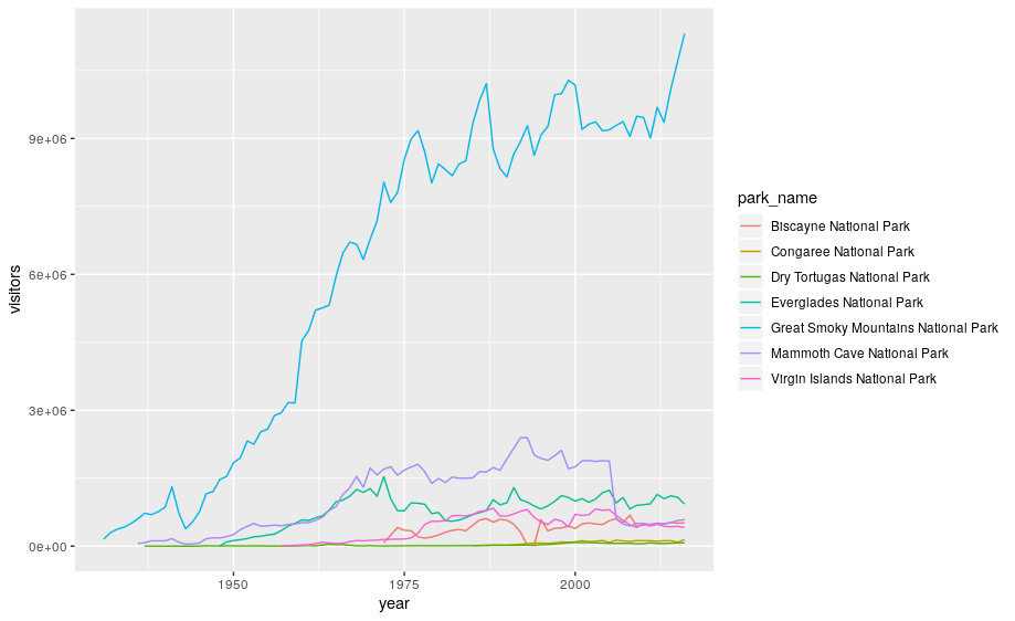
None of these are great for visualizing data over time. We can use geom_line() in the same way we used geom_point.
ggplot(se, aes(x = year, y = visitors, color = park_name)) +
   geom_line()
ggplot2 provides over 30 geoms, and extension packages provide even more (see https://exts.ggplot2.tidyverse.org/ for a sampling). The best way to get a comprehensive overview is the ggplot2 cheatsheet. To learn more about any single geom, use help: ?geom_smooth.
To display multiple geoms in the same plot, add multiple geom functions to ggplot():
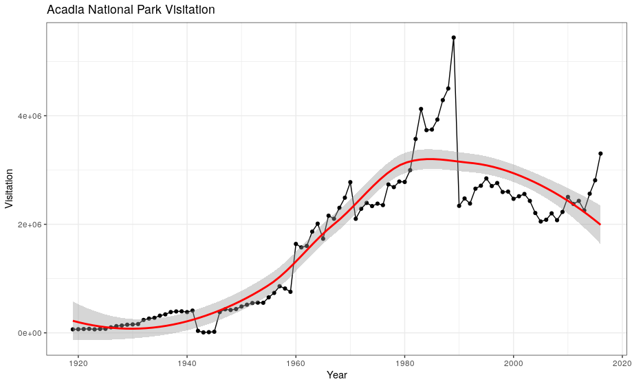
geom_smooth allows you to view a smoothed mean of data. Here we look at the smooth mean of visitation over time to Acadia National Park:
ggplot(data = acadia) +
  geom_point(aes(x = year, y = visitors)) +
  geom_line(aes(x = year, y = visitors)) +
  geom_smooth(aes(x = year, y = visitors)) +
  labs(title = "Acadia National Park Visitation",
       y = "Visitation",
       x = "Year") +
  theme_bw()
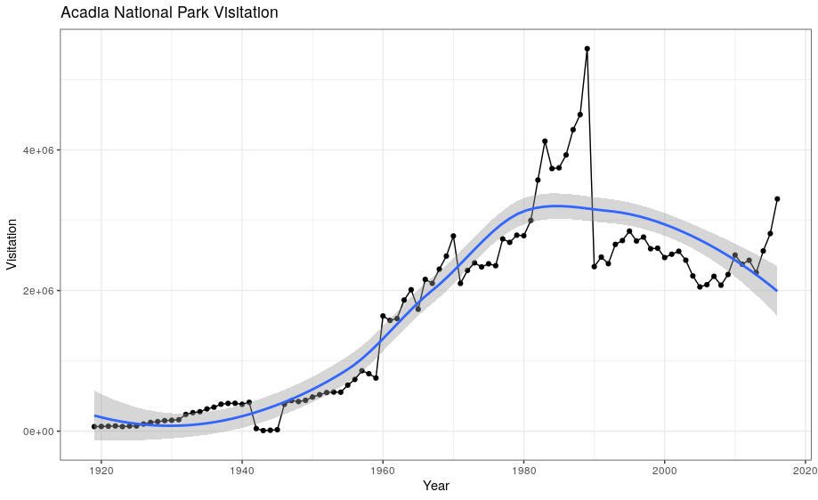
Notice that this plot contains three geoms in the same graph! Each geom is using the set of mappings in the first line. ggplot2 will treat these mappings as global mappings that apply to each geom in the graph.
If you place mappings in a geom function, ggplot2 will treat them as local mappings for the layer. It will use these mappings to extend or overwrite the global mappings for that layer only. This makes it possible to display different aesthetics in different layers.
ggplot(data = acadia, aes(x = year, y = visitors)) +
  geom_point() +
  geom_line() +
  geom_smooth(color = "red") +
  labs(title = "Acadia National Park Visitation",
       y = "Visitation",
       x = "Year") +
  theme_bw()
Exercise
With all of this information in hand, please take another five minutes to either improve one of the plots generated in this exercise or create a beautiful graph of your own. Use the RStudio
ggplot2cheat sheet for inspiration.Here are some ideas:
- See if you can change the thickness of the lines or line type (e.g. dashed line)
- Can you find a way to change the name of the legend? What about its labels?
- Try using a different color palette: see the R Cookbook.
4. Bar charts
Next, let’s take a look at a bar chart. Bar charts seem simple, but they are interesting because they reveal something subtle about plots. Consider a basic bar chart, as drawn with geom_bar(). The following chart displays the total number of parks in each state within the Pacific West region.
ggplot(data = visit_16, aes(x = state)) +
  geom_bar()
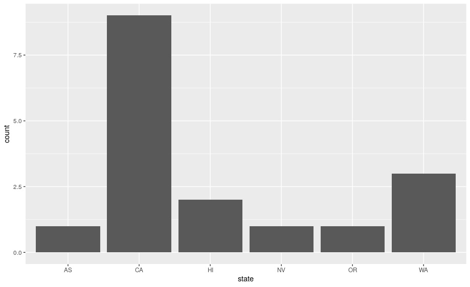
On the x-axis, the chart displays state, a variable from visit_16. On the y-axis, it displays count, but count is not a variable in visit_16! Where does count come from? Many graphs, like scatterplots, plot the raw values of your dataset. Other graphs, like bar charts, calculate new values to plot:
-
bar charts, histograms, and frequency polygons bin your data and then plot bin counts, the number of points that fall in each bin.
-
smoothers fit a model to your data and then plot predictions from the model.
-
boxplots compute a robust summary of the distribution and then display a specially formatted box.
The algorithm used to calculate new values for a graph is called a stat, short for statistical transformation.
You can learn which stat a geom uses by inspecting the default value for the stat argument. For example, ?geom_bar shows that the default value for stat is “count”, which means that geom_bar() uses stat_count(). stat_count() is documented on the same page as geom_bar(), and if you scroll down you can find a section called “Computed variables”. That describes how it computes two new variables: count and prop.
ggplot2 provides over 20 stats for you to use. Each stat is a function, so you can get help in the usual way, e.g. ?stat_bin. To see a complete list of stats, try the ggplot2 cheatsheet.
4.1 Position adjustments
There’s one more piece of magic associated with bar charts. You can colour a bar chart using either the color aesthetic, or, more usefully, fill:
ggplot(data = visit_16, aes(x = state, y = visitors, fill = park_name)) +
  geom_bar(stat = "identity")
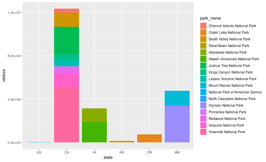
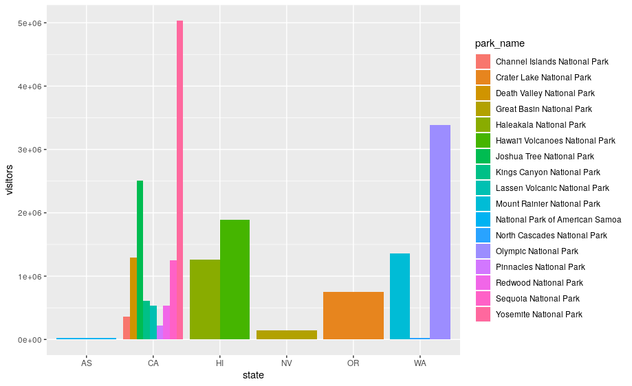
The stacking is performed automatically by the position adjustment specified by the position argument. If you don’t want a stacked bar chart, you can use "dodge".
position = "dodge"places overlapping objects directly beside one another. This makes it easier to compare individual values.
ggplot(data = visit_16, aes(x = state, y = visitors, fill = park_name)) +
  geom_bar(stat = "identity", position = "dodge")
Exercise
With all of this information in hand, please take another five minutes to either improve one of the plots generated in this exercise or create a beautiful graph of your own. Use the RStudio
ggplot2cheat sheet for inspiration. Remember to use the help documentation (e.g.?geom_bar) Here are some ideas:
- Flip the x and y axes.
- Change the color palette used
- Use
scale_x_discreteto change the x-axis tick labels to the full state names (Arizona, Colorado, etc.)- Make a bar chart using the Massachussets dataset (
mass) and find out how many parks of each type are in the state.Solution
# 1) flip the x and y axes
ggplot(data = visit_16, aes(x = state, y = visitors, fill = park_name)) +
  geom_bar(stat = "identity", position = "dodge") +
  coord_flip()
# 2) change the color palette ggplot(data = visit_16, aes(x = state, y = visitors, fill = park_name)) + geom_bar(stat = "identity", position = "dodge") + coord_flip() + scale_fill_brewer(palette = "Set3")# 3) change x-axis tick labels ggplot(data = visit_16, aes(x = state, y = visitors, fill = park_name)) + geom_bar(stat = "identity", position = "dodge") + coord_flip() + scale_fill_brewer(palette = "Set3") + scale_x_discrete(labels = mass$park_name)# 4) How many of each types of parks are in Massachusetts? ggplot(data = mass) + geom_bar(aes(x = type, fill = type)) + labs(x = "Type of park", y = "Number of parks")+ theme(axis.text.x = element_text(angle = 45, hjust = 1, size = 7))
4.2 Arranging and exporting plots
After creating your plot, you can save it to a file in your favorite format. The Export tab in the Plot pane in RStudio will save your plots at low resolution, which will not be accepted by many journals and will not scale well for posters.
Instead, use the ggsave() function, which allows you easily change the dimension and resolution of your plot by adjusting the appropriate arguments (width, height and dpi):
my_plot <- ggplot(data = mass) +
      geom_bar(aes(x = type, fill = park_name)) +
  labs(x = "",
       y = "")+
  theme(axis.text.x = element_text(angle = 45, hjust = 1, size = 7))

ggsave("name_of_file.png", my_plot, width = 15, height = 10)
Note: The parameters width and height also determine the font size in the saved plot.
4.3 bonus 1: animated graph
So as you can see, ggplot2 is a fantastic package for visualizing data. But there are some additional packages that let you make plots interactive. plotly, gganimate.
# install package if necessary and load library
# install.packages("plotly")
library(plotly)

my_plot <- ggplot(data = mass) +
      geom_bar(aes(x = type, fill = park_name)) +
  labs(x = "",
       y = "")+
  theme(axis.text.x = element_text(angle = 45, hjust = 1, size = 7))

ggplotly(my_plot)
acad_vis <- ggplot(data = acadia, aes(x = year, y = visitors)) +
  geom_point() +
  geom_line() +
  geom_smooth(color = "red") +
  labs(title = "Acadia National Park Visitation",
       y = "Visitation",
       x = "Year") +
  theme_bw()

ggplotly(acad_vis)
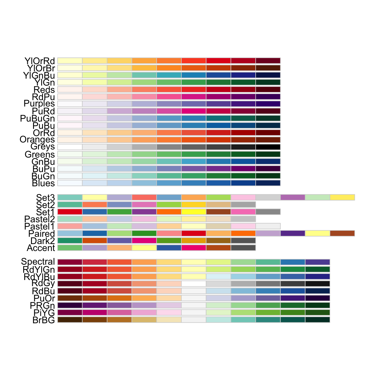
4.4 bonus 2: additional colours with scale_colour_brewer
We can use the scale_colour_brewer from the ggplot2 package to change the colour scheme of our plot.
From the help page of the function:
The brewer scales provides sequential, diverging and qualitative colour schemes from ColorBrewer. These are particularly well suited to display discrete values on a map. See http://colorbrewer2.org for more information.
ggplot(data = ca, aes(x = year, y = visitors, color = park_name)) +
  geom_point() +
  geom_line() +
  labs(title = "Acadia National Park Visitation",
       y = "Visitation",
       x = "Year") +
  theme_bw() +
  scale_colour_brewer(type = "qual", palette = "Set1")
All palettes are visible below. Always make sure that you have enough colors in the palette for the number of categories you want to display.
5. Resources
Here are some additional resources for data visualization in R:
- ggplot2-cheatsheet-2.1.pdf
- Interactive Plots and Maps - Environmental Informatics
- Graphs with ggplot2 - Cookbook for R
- ggplot2 Essentials - STHDA
- “Why I use ggplot2” - David Robinson Blog Post
- “The Grammar of Graphics explained” - Towards Data Science blog series
Key Points
ggplot2relies on the grammar of graphics, an advanced methodology to visualise data.ggplot() creates a coordinate system that you can add layers to.
You pass a mapping using
aes()to link dataset variables to visual properties.You add one or more layers (or
geoms) to theggplotcoordinate system andaesmapping.Building a minimal plot requires to supply a dataset, mapping aesthetics and geometric layers (geoms).
ggplot2offers advanced graphical visualisations to plot extra information from the dataset.
Data transformation with dplyr
Overview
Teaching: 45 min
Exercises: 15 minQuestions
How do I perform data transformations such as removing columns on my data using R?
What are tidy data (in opposition to messy data)?
How do I import data into R (e.g. from a web link)?
How can I make my code more readable when performing a series of transformation?
Objectives
Learn how to explore a publically available dataset (gapminder).
Learn how to perform data transformation with the
dplyrfunctions from thetidyversepackage
![]()
Table of contents
- 1. Introduction
- 2. Explore the gapminder dataframe
- 3.
dplyrbasics - 4. All together now
- 5. Joining datasets
- 6. Resources and credits
1. Introduction
1.1 Why should we care about data transformation?
Data scientists, according to interviews and expert estimates, spend from 50 percent to 80 percent of their time mired in the mundane labor of collecting and preparing data, before it can be explored for useful information. - NYTimes (2014)
What are some common things you like to do with your data? Maybe remove rows or columns, do calculations and maybe add new columns? This is called data wrangling (or more simply data transformation). It’s not data management or data manipulation: you keep the raw data raw and do these things programatically in R with the tidyverse.
We are going to introduce you to data wrangling in R first with the tidyverse. The tidyverse is a new suite of packages that match a philosophy of data science developed by Hadley Wickham and the RStudio team. I find it to be a more straight-forward way to learn R. We will also show you by comparison what code will look like in base-R, which means, in R without any additional packages (like the tidyverse package) installed. I like David Robinson’s blog post on the topic of teaching the tidyverse first.
For some things, base-R is more straightforward, and we’ll show you that too. Whenever we use a function that is from the tidyverse, we will prefix it so you’ll know for sure.
1.2 Gapminder dataset
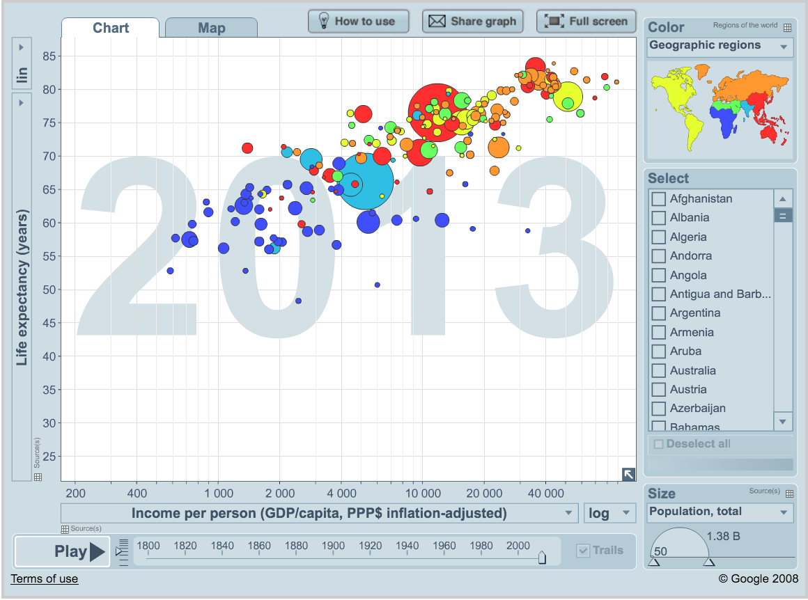
We’ll be using Gapminder data, which represents the health and wealth of nations. It was pioneered by Hans Rosling, who is famous for describing the prosperity of nations over time through famines, wars and other historic events with this beautiful data visualization in his 2006 TED Talk: The best stats you’ve ever seen:
1.3 Load the tidyverse suite
We’ll use the package dplyr, which is bundled within the tidyverse suite of packages. Please load the tidyverse if not already done.
library("tidyverse")
The tidyverse package suite contains all the tools you need for data science. Actually, Hadley Wickham and RStudio have created a ton of packages that help you at every step of the way here. This is from one of Hadley’s presentations:
1.4 Create a new R Markdown file.
We’ll do this in a new R Markdown file.
Here’s what to do:
- Clear your workspace (Session > Restart R)
- New File > R Markdown…
- Save as
gapminder-wrangle.Rmd - Delete the irrelevant text and write a little note to yourself about this section: “cleaning and transforming the gapminder dataset.”
2. Explore the gapminder dataframe
Previously, we explored the national parks dataframe visually. Today, we’ll explore a dataset by the numbers. We will work with some of the data from the Gapminder project.
The data are on GitHub. Navigate to: https://github.com/carpentries-incubator/open-science-with-r/blob/gh-pages/data/gapminder.csv.
This is data-view mode: so we can have a quick look at the data. It’s a .csv file, which you’ve probably encountered before, but GitHub has formatted it nicely so it’s easy to look at. You can see that for every country and year, there are several columns with data in them.
2.1 Import data with readr::read_csv()
We can read this data into R directly from GitHub, without downloading it. But we can’t read this data in view-mode. We have to click on the Raw button on the top-right of the data. This displays it as the raw csv file, without formatting.
Copy the url for raw data: https://raw.githubusercontent.com/carpentries-incubator/open-science-with-r/gh-pages/data/gapminder.csv
Now, let’s go back to RStudio. In our R Markdown, let’s read this .csv file and name the variable gapminder. We will use the read_csv() function from the readr package (part of the tidyverse, so it’s already installed!).
## read gapminder csv. Note the readr:: prefix identifies which package it's in
gapminder <- readr::read_csv('https://raw.githubusercontent.com/carpentries-incubator/open-science-with-r/gh-pages/data/gapminder.csv')
Note
read_csvworks with local filepaths as well, you could use one from your computer.
2.2 Dataset inspection
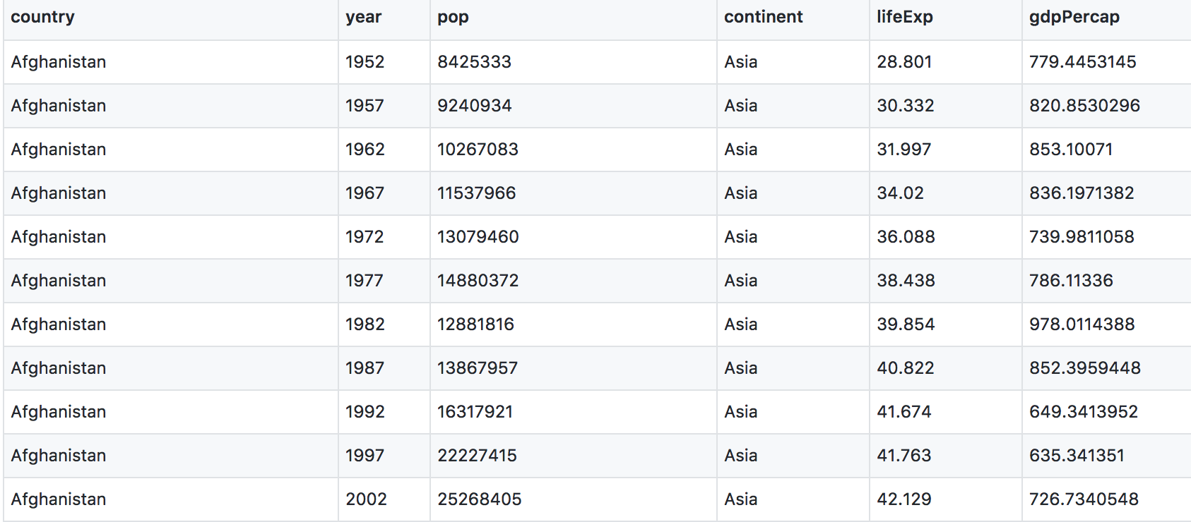
Let’s inspect the data with head and tail:
head(gapminder) # shows first 6
tail(gapminder) # shows last 6

head(gapminder, n = 10) # shows first X that you indicate
tail(gapminder, n = 12) # guess what this does!
str() will provide a sensible description of almost anything: when in doubt, inspect using str() on some of the recently created objects to get some ideas about what to do next.
str(gapminder) # ?str - displays the structure of an object
 str(gapminder)
Classes ‘spec_tbl_df’, ‘tbl_df’, ‘tbl’ and 'data.frame':	1704 obs. of  6 variables:
 $ country  : chr  "Afghanistan" "Afghanistan" "Afghanistan" "Afghanistan" ...
 $ year     : num  1952 1957 1962 1967 1972 ...
 $ pop      : num  8425333 9240934 10267083 11537966 13079460 ...
 $ continent: chr  "Asia" "Asia" "Asia" "Asia" ...
 $ lifeExp  : num  28.8 30.3 32 34 36.1 ...
 $ gdpPercap: num  779 821 853 836 740 ...
 - attr(*, "spec")=
  .. cols(
  ..   country = col_character(),
  ..   year = col_double(),
  ..   pop = col_double(),
  ..   continent = col_character(),
  ..   lifeExp = col_double(),
  ..   gdpPercap = col_double()
  .. )
This will show how R understood your data types. Check that numbers are indeed understood as num/numeric and strings as chr/character.
You can get the number of rows and columns of the gapminder dataframe with dim().
dim(gapminder)
[1] 1704 6
It shows that our dataframe has 1704 rows and 6 columns.
R imports gapminder as a dataframe. We aren’t going to get into the other types of data receptacles today (‘arrays’, ‘matrices’), because working with dataframes is what you should primarily use. Why?
- dataframes contain related variables neatly together, great for analysis
- most functions, including the latest and greatest packages actually require that your data be in a dataframe
- dataframes can hold variables of different flavors such as:
- character data (country or continent names; “Characters (chr)”)
- quantitative data (years, population; “Integers (int)” or “Numeric (num)”)
- categorical information (male vs. female)
We can also see the gapminder variable in RStudio’s Environment pane (top right).
More ways to learn basic info on a dataframe.
names(gapminder)  # column names
ncol(gapminder)   # ?ncol number of columns
nrow(gapminder)   # ?nrow number of rows
2.3 Descriptive statistics of the gapminder dataset
A statistical overview can be obtained with summary(), or with skimr::skim()
summary(gapminder)
   country               year           pop             continent            lifeExp        gdpPercap
 Length:1704        Min.   :1952   Min.   :6.001e+04   Length:1704        Min.   :23.60   Min.   :   241.2
 Class :character   1st Qu.:1966   1st Qu.:2.794e+06   Class :character   1st Qu.:48.20   1st Qu.:  1202.1
 Mode  :character   Median :1980   Median :7.024e+06   Mode  :character   Median :60.71   Median :  3531.8
                    Mean   :1980   Mean   :2.960e+07                      Mean   :59.47   Mean   :  7215.3
                    3rd Qu.:1993   3rd Qu.:1.959e+07                      3rd Qu.:70.85   3rd Qu.:  9325.5
                    Max.   :2007   Max.   :1.319e+09                      Max.   :82.60   Max.   :113523.1
This will give simple descriptive statistics (e.g. median, average) for each column if numeric.
Finally, the skimr package provides a powerful descriptive function for dataframes.
library(skimr)
skim(gapminder)
── Data Summary ────────────────────────
                           Values
Name                       gapminder
Number of rows             1704
Number of columns          6
_______________________
Column type frequency:
  character                2
  numeric                  4
________________________
Group variables            None

── Variable type: character ──────────────────────────────────────────────────────────────────────────────────────────────────────────────
  skim_variable n_missing complete_rate   min   max empty n_unique whitespace
1 country               0             1     4    24     0      142          0
2 continent             0             1     4     8     0        5          0

── Variable type: numeric ────────────────────────────────────────────────────────────────────────────────────────────────────────────────
  skim_variable n_missing complete_rate       mean          sd      p0       p25       p50        p75         p100 hist
1 year                  0             1     1980.         17.3  1952      1966.     1980.      1993.        2007   ▇▅▅▅▇
2 pop                   0             1 29601212.  106157897.  60011   2793664   7023596.  19585222.  1318683096   ▇▁▁▁▁
3 lifeExp               0             1       59.5        12.9    23.6      48.2      60.7       70.8         82.6 ▁▆▇▇▇
4 gdpPercap             0             1     7215.       9857.    241.     1202.     3532.      9325.      113523.  ▇▁▁▁▁
This gives you a comprehensive view of your data at a glance.
3. dplyr basics
OK, so let’s start wrangling with the dplyr collection of functions. .
There are five dplyr functions that you will use to do the vast majority of data manipulations:
-
filter(): pick observations by their values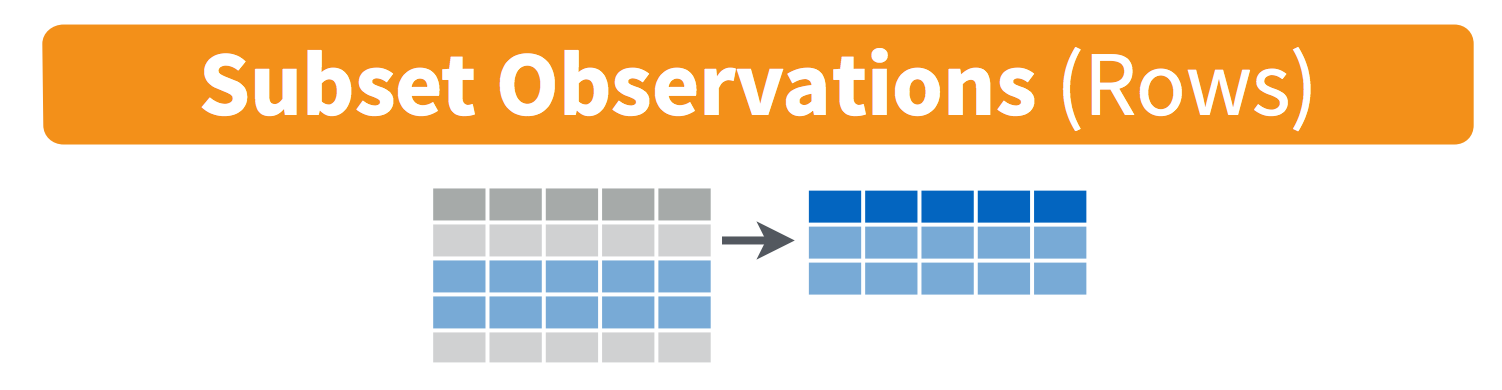
-
select(): pick variables by their names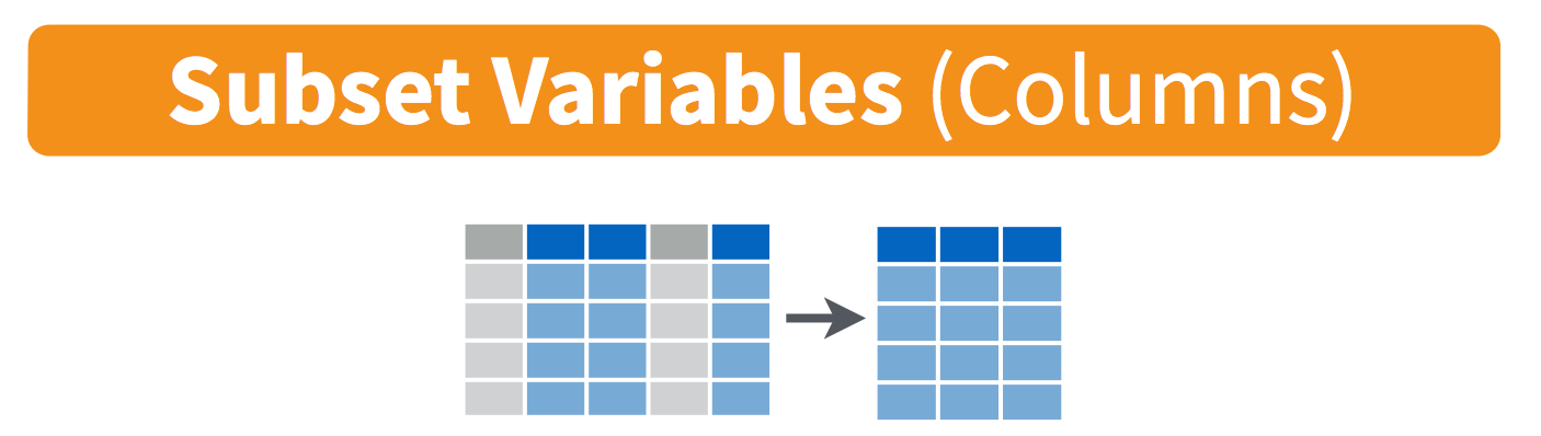
-
mutate(): create new variables with functions of existing variables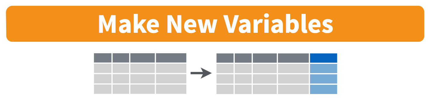
-
summarise(): collapse many values down to a single summary
-
arrange(): reorder the rows
These can all be used in conjunction with group_by() which changes the scope of each function from operating on the entire dataset to operating on it group-by-group. These six functions provide the verbs for a language of data manipulation.
All verbs work similarly:
- The first argument is a data frame.
- The subsequent arguments describe what to do with the data frame. You can refer to columns in the data frame directly without using
$. - The result is a new data frame.
Together these properties make it easy to chain together multiple simple steps to achieve a complex result.
3.1 filter() observations
You will want to isolate bits of your data; maybe you want to only look at a single country or a few years. R calls this subsetting.
filter() is a function in dplyr that takes logical expressions and returns the rows for which all are TRUE.
Visually, we are doing this:
Remember your logical expressions from this morning? We’ll use < and == here.
filter(gapminder, lifeExp < 29)
You can say this out loud: “Filter the gapminder data for life expectancy less than 29”. Notice that when we do this, all the columns are returned, but only the rows that have the life expectancy less than 29. We’ve subsetted by row.
Let’s try another: “Filter the gapminder data for the country Mexico”.
filter(gapminder, country == "Mexico")
How about if we want two country names? We can’t use the == operator here, because it can only operate on one thing at a time. We will use the %in% operator:
filter(gapminder, country %in% c("Mexico", "Peru"))
How about if we want Mexico in 2002? You can pass filter different criteria:
filter(gapminder, country == "Mexico", year == 2002)
Exercise
What is the mean life expectancy of Sweden?
Hint: do this in 2 steps by assigning a variable and then using themean()function.Solution
sweden <- filter(gapminder, country == "Sweden")
mean(sweden$lifeExp)
3.2 select() variables
We use select() to subset the data on variables or columns.
Visually, we are doing this:
We can select multiple columns with a comma, after we specify the data frame (gapminder).
select(gapminder, year, lifeExp)
We can also use - to deselect columns
select(gapminder, -continent, -lifeExp) # you can use - to deselect columns
3.3 The pipe %>% operator
What if we want to use select() and filter() together?
Let’s filter for Cambodia and remove the continent and lifeExp columns. We’ll save this as a variable. Actually, as two temporary variables, which means that for the second one we need to operate on gap_cambodia, not gapminder.
gap_cambodia  <- filter(gapminder, country == "Cambodia")
gap_cambodia2 <- select(gap_cambodia, -continent, -lifeExp)
We also could have called them both gap_cambodia and overwritten the first assignment. Either way, naming them and keeping track of them gets super cumbersome, which means more time to understand what’s going on and opportunities for confusion or error.
Good thing there is an awesome alternative.
Before we go any further, we should exploit the new pipe operator that comes from the magrittr package by Stefan Bache. The package name refers to the Belgium surrealist artist René Magritte that made a famous painting with a pipe.

The %>% operator is going to change your life. You no longer need to enact multi-operation commands by nesting them inside each other. And we won’t need to make temporary variables like we did in the Cambodia example above. This new syntax leads to code that is much easier to write and to read: it actually tells the story of your analysis.
Here’s what it looks like: %>%.
Keyboard shortcuts for the pipe operator
The RStudio keyboard shortcut:
Ctrl+Shift+M(Windows),Cmd+Shift+M(Mac).
Let’s demo then I’ll explain:
gapminder %>% head()
# A tibble: 6 x 6
  country      year      pop continent lifeExp gdpPercap
  <chr>       <dbl>    <dbl> <chr>       <dbl>     <dbl>
1 Afghanistan  1952  8425333 Asia         28.8      779.
2 Afghanistan  1957  9240934 Asia         30.3      821.
3 Afghanistan  1962 10267083 Asia         32.0      853.
4 Afghanistan  1967 11537966 Asia         34.0      836.
5 Afghanistan  1972 13079460 Asia         36.1      740.
6 Afghanistan  1977 14880372 Asia         38.4      786.
This is equivalent to head(gapminder).
This pipe operator takes the thing on the left-hand-side and pipes it into the function call on the right-hand-side. It literally drops it in as the first argument.
Never fear, you can still specify other arguments to this function! To see the first 3 rows of Gapminder, we could say head(gapminder, n = 3) or this:
gapminder %>% head(n = 3)
I’ve advised you to think “gets” whenever you see the assignment operator, <-. Similarly, you should think “and then” whenever you see the pipe operator, %>%.
One of the most awesome things about this is that you START with the data before you say what you’re doing to DO to it. So above: “take the gapminder data, and then give me the first three entries”.
This means that instead of this:
## instead of this...
gap_cambodia  <- filter(gapminder, country == "Cambodia")
gap_cambodia2 <- select(gap_cambodia, -continent, -lifeExp)

## ...we can do this
gap_cambodia  <- gapminder %>% filter(country == "Cambodia")
gap_cambodia2 <- gap_cambodia %>% select(-continent, -lifeExp)
So you can see that we’ll start with gapminder in the first example line, and then gap_cambodia in the second. This makes it a bit easier to see what data we are starting with and what we are doing to it.
Exercise
Can you filter for Finland and show only the
pop(population) column?
Use the pipe%>%operator twice.Solution
gapminder %>% filter(country == "Finland") %>% select(pop)
We can use the pipe to chain those two operations together:
gap_cambodia  <- gapminder %>% filter(country == "Cambodia") %>%
  select(-continent, -lifeExp)
What’s happening here? In the second line, we were able to delete gap_cambodia2 <- gap_cambodia, and put the pipe operator above. This is possible since we wanted to operate on the gap_cambodia data anyways. And we weren’t truly excited about having a second variable named gap_cambodia2 anyways, so we can get rid of it. This is huge, because most of your data wrangling will have many more than 2 steps, and we don’t want a gap_cambodia14!
Let’s write it again but using multiple lines so it’s nicer to read.
gap_cambodia  <- gapminder %>%
  filter(country == "Cambodia") %>%
  select(-continent, -lifeExp)
Amazing. I can actually read this like a story and there aren’t temporary variables that get super confusing. In my head:
start with the
gapminderdata, and then
filter for Cambodia, and then
deselect the variables continent and lifeExp.
Being able to read a story out of code like this is really game-changing. We’ll continue using this syntax as we learn the other dplyr verbs.
3.4 mutate() adds new variables
Alright, let’s keep going.
Let’s say we need to compute a new variable from two pre-existing variables in the dataframe. We could calculate the Gross Domestic Product from the gdpPercap (GDP per person) and the pop (population) variables.
Visually, we are doing this:
We will name our new column gdp and assign it with a single =.
gapminder %>%
  mutate(gdp = pop * gdpPercap)
   country      year      pop continent lifeExp gdpPercap          gdp
   <chr>       <dbl>    <dbl> <chr>       <dbl>     <dbl>        <dbl>
 1 Afghanistan  1952  8425333 Asia         28.8      779.  6567086330.
 2 Afghanistan  1957  9240934 Asia         30.3      821.  7585448670.
 3 Afghanistan  1962 10267083 Asia         32.0      853.  8758855797.
 4 Afghanistan  1967 11537966 Asia         34.0      836.  9648014150.
 5 Afghanistan  1972 13079460 Asia         36.1      740.  9678553274.
 6 Afghanistan  1977 14880372 Asia         38.4      786. 11697659231.
 7 Afghanistan  1982 12881816 Asia         39.9      978. 12598563401.
 8 Afghanistan  1987 13867957 Asia         40.8      852. 11820990309.
 9 Afghanistan  1992 16317921 Asia         41.7      649. 10595901589.
10 Afghanistan  1997 22227415 Asia         41.8      635. 14121995875.
This is quite handy when you need to calculate a percentage for example.
Exercise
Find the maximum gdpPercap of Egypt and the maximum gdpPercap of Vietnam. Create a new column with
mutate().
Hint: usemax().Solution
Egypt:
gapminder %>%
select(-continent, -lifeExp) %>%(not super necessary but to simplify)
filter(country == "Egypt") %>%
mutate(gdp = pop * gdpPercap) %>%
mutate(max_gdp = max(gdp))Vietnam:
gapminder %>%
select(-continent, -lifeExp) %>%(not super necessary but to simplify)
filter(country == "Vietnam") %>%
mutate(gdp = pop * gdpPercap, max_gdp = max(gdp))(multiple variables created)
With the things we know so far, the answers you have are maybe a bit limiting. First, we had to act on Egypt and Vietnam separately, and repeat the same code. Copy-pasting like this is also super error prone.
And second, this max_gdpPercap column is pretty redundant, because it’s a repeated value a ton of times. Sometimes this is exactly what you want! You are now set up nicely to maybe take a proportion of gdpPercap/max_gdpPercap for each year or something. But maybe you only wanted that max_gdpPercap for something else. Let’s keep going…
3.5 group_by makes group that can be summarize()
group_by operates on groups
Let’s tackle that first issue first. So how do we less painfully calculate the max gdpPercap for all countries?
Visually, we are doing this:
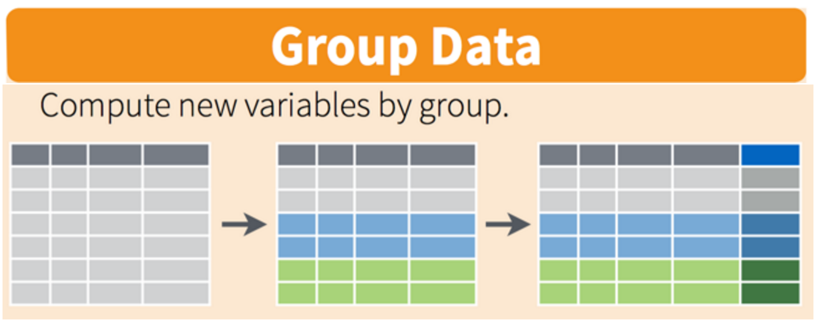
gapminder %>%
  group_by(country) %>%
  mutate(gdp = pop * gdpPercap, max_gdp = max(gdp)) %>%
  ungroup() # if you use group_by, also use ungroup() to save heartache later
The ungroup() serves to allow operations again (mutate or summarize) on the grouping variables. If you would like to change something on country you would need to ungroup() them first. For an extensive discussion about ungroup, see the RStudio community forum here.
So instead of filtering for a specific country, we’ve grouped by country, and then done the same operations. It’s hard to see; let’s look at a bunch at the tail:
gapminder %>%
  group_by(country) %>%
  mutate(gdp = pop * gdpPercap,
  	     max_gdp = max(gdp)) %>%
  ungroup() %>%
  tail(30)
 country     year      pop continent lifeExp gdpPercap          gdp      max_gdp
   <chr>      <dbl>    <dbl> <chr>       <dbl>     <dbl>        <dbl>        <dbl>
 1 Yemen Rep.  1982  9657618 Asia         49.1     1978. 19098490176. 50659874994.
 2 Yemen Rep.  1987 11219340 Asia         52.9     1972. 22121638707. 50659874994.
 3 Yemen Rep.  1992 13367997 Asia         55.6     1879. 25125105886. 50659874994.
 4 Yemen Rep.  1997 15826497 Asia         58.0     2117. 33512362498. 50659874994.
 5 Yemen Rep.  2002 18701257 Asia         60.3     2235. 41793958635. 50659874994.
 6 Yemen Rep.  2007 22211743 Asia         62.7     2281. 50659874994. 50659874994.
 7 Zambia      1952  2672000 Africa       42.0     1147.  3065822956. 14931695864.
 8 Zambia      1957  3016000 Africa       44.1     1312.  3956861606. 14931695864.
 9 Zambia      1962  3421000 Africa       46.0     1453.  4969774845. 14931695864.
10 Zambia      1967  3900000 Africa       47.8     1777.  6930601540. 14931695864.
OK, this is great. But what if this what we needed, a max_gdp value for each country. We don’t need that kind of repeated value for each of the max_gdp values. Here’s the next function:
summarize() compiles values for each group
We want to operate on a group, but actually collapse or distill the output from that group. The summarize() function will do that for us.
Visually, we are doing this:
Here we go:
gapminder %>%
  group_by(country) %>%
  mutate(gdp = pop * gdpPercap) %>%
  summarize(max_gdp = max(gdp)) %>%
  ungroup()
  country           max_gdp
   <chr>               <dbl>
 1 Afghanistan  31079291949.
 2 Albania      21376411360.
 3 Algeria     207444851958.
 4 Angola       59583895818.
 5 Argentina   515033625357.
 6 Australia   703658358894.
 7 Austria     296229400691.
 8 Bahrain      21112675360.
 9 Bangladesh  209311822134.
10 Belgium     350141166520.
How cool is that! summarize() will actually only keep the columns that are grouped_by or summarized. So if we wanted to keep other columns, we’d have to do have a few more steps.
3.6 arrange() orders columns
This is ordered alphabetically, which is cool. But let’s say we wanted to order it in ascending order for max_gdp. The dplyr function is arrange().
gapminder %>%
  group_by(country) %>%
  mutate(gdp = pop * gdpPercap) %>%
  summarize(max_gdp = max(gdp)) %>%
  ungroup() %>%
  arrange(max_gdp)
   country                      max_gdp
   <chr>                          <dbl>
 1 Sao Tome and Principe     319014077.
 2 Comoros                   701111696.
 3 Guinea-Bissau             950984749.
 4 Djibouti                 1033689705.
 5 Gambia                   1270911775.
 6 Liberia                  1495937378.
 7 Central African Republic 3084613079.
 8 Lesotho                  3158513357.
 9 Burundi                  3669693671.
10 Eritrea                  3707155863.
Your turn
Exercise
- Arrange your data frame in descending order (opposite of what we’ve done). Look at the documentation
?arrange- Find the maximum life expectancy for countries in Asia. What is the earliest year you encounter? The latest? Hint: you can use either
base::maxordplyr::arrange()…Solution
1)
arrange(desc(max_gdp))2)gapminder %>%filter(continent == 'Asia') %>%group_by(country) %>%filter(lifeExp == max(lifeExp)) %>%arrange(year)
4. All together now
We have done a pretty incredible amount of work in a few lines. Our whole analysis is this. Imagine the possibilities from here. It’s very readable: you see the data as the first thing, it’s not nested. Then, you can read the verbs. This is the whole thing, with explicit package calls from readr:: and dplyr::
4.1 With dplyr
# load libraries
library(tidyverse)

# read in data
gapminder <- readr::read_csv('https://raw.githubusercontent.com/carpentries-incubator/open-science-with-r/gh-pages/data/gapminder.csv')

## summarize
gap_max_gdp <- gapminder %>%
  dplyr::select(-continent, -lifeExp) %>% # or select(country, year, pop, gdpPercap)
  dplyr::group_by(country) %>%
  dplyr::mutate(gdp = pop * gdpPercap) %>%
  dplyr::summarize(max_gdp = max(gdp)) %>%
  dplyr::ungroup()
I actually am borrowing this “All together now” from Tony Fischetti’s blog post How dplyr replaced my most common R idioms. With that as inspiration, this is how what we have done would look like in Base R.
4.2 With base R
Let’s compare with some base R code to accomplish the same things. Base R requires subsetting with the [rows, columns] notation. This notation is something you’ll see a lot in base R. the brackets [ ] allow you to extract parts of an object. Within the brackets, the comma separates rows from columns.
If we don’t write anything after the comma, that means “all columns”. And if we don’t write anything before the comma, that means “all rows”.
Also, the $ operator is how you access specific columns of your dataframe. You can also add new columns like we will do with mex$gdp below.
Instead of calculating the max for each country like we did with dplyr above, here we will calculate the max for one country, Mexico. Tomorrow we will learn how to do it for all the countries, like we did with dplyr::group_by().
## gapminder-wrangle.R --- baseR
## J. Lowndes lowndes@nceas.ucsb.edu

gapminder <- read.csv('https://raw.githubusercontent.com/carpentries-incubator/open-science-with-r/gh-pages/data/gapminder.csv', stringsAsFactors = FALSE)
x1  <- gapminder[ , c('country', 'year', 'pop', 'gdpPercap') ] # subset columns
mex <- x1[x1$country == "Mexico", ] # subset rows
mex$gdp <- mex$pop * mex$gdpPercap # add new columns
mex$max_gdp <- max(mex$gdp)
Note too that the chain operator %>% that we used with the tidyverse lets us get away from the temporary variable x1.
Discussion
What do you personally favor? What are pros and cons of the
dplyrandbasemethods?
Bothdplyrandbasesolutions are fine. In the long run, you might better understand the pros and cons of each method.
5. Joining datasets
We’ve learned a ton in this session and we may not get to this right now. If we don’t have time, we’ll start here before getting into the next chapter: tidyr.
5.1 Types of join
Most of the time you will have data coming from different places or in different files, and you want to put them together so you can analyze them. Datasets you’ll be joining can be called relational data, because it has some kind of relationship between them that you’ll be acting upon. In the tidyverse, combining data that has a relationship is called “joining”.
From the RStudio cheatsheet (note: this is an earlier version of the cheatsheet but I like the graphics):
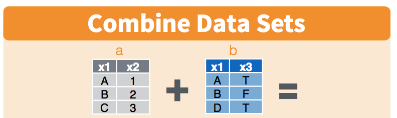
Let’s have a look at this and pretend that the x1 column is a study site and x2 is the variables we’ve recorded (like species count) and x3 is data from an instrument (like temperature data). Notice how you may not have exactly the same observations in the two datasets: in the x1 column, observations A and B appear in both datasets, but notice how the table on the left has observation C, and the table on the right has observation D.
If you wanted to combine these two tables, how would you do it? There are some decisions you’d have to make about what was important to you. The cheatsheet visualizes it for us:
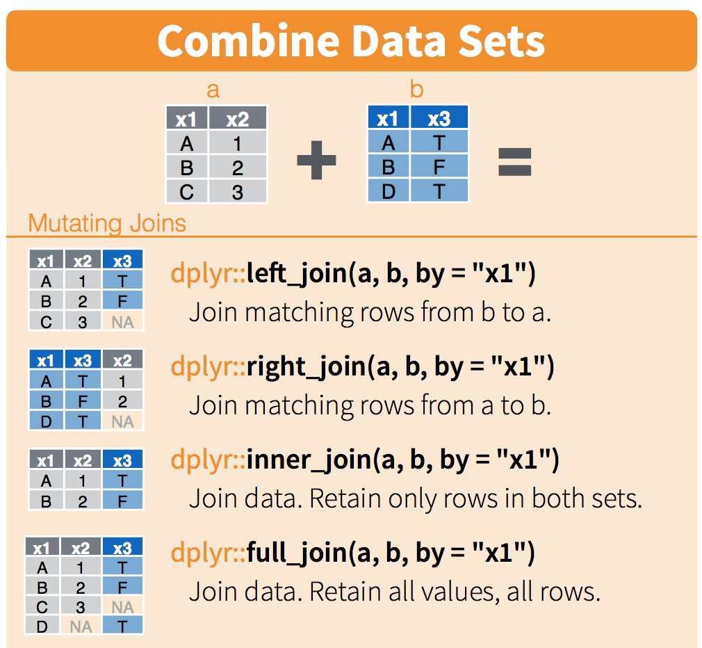
We will only talk about this briefly here, but you can refer to this more as you have your own datasets that you want to join. This describes the figure above::
left_joinkeeps everything from the left table and matches as much as it can from the right table. In R, the first thing that you type will be the left table (because it’s on the left)right_joinkeeps everything from the right table and matches as much as it can from the left tableinner_joinonly keeps the observations that are similar between the two tablesfull_joinkeeps all observations from both tables.
I like graphical representations of complex things so here’s a nice one taken from a blog post:
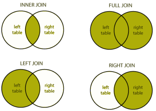
You can visualise the different outputs from the different joins.
5.2 Join the gapminder dataset with a co2 dataset
Let’s play with these CO2 emissions data to illustrate:
## read in the data.
co2 <- read_csv("https://raw.githubusercontent.com/carpentries-incubator/open-science-with-r/gh-pages/data/co2.csv")

## explore
co2 %>% head()
# A tibble: 6 x 2
  country        co2_2007
  <chr>             <dbl>
1 Afghanistan      2938.
2 Albania          4218.
3 Algeria        105838.
4 American Samoa     18.4
5 Angola          17405.
6 Anguilla           12.4
It is a simple dataframe with countries and their level of CO2 in 2007.
Let’s filter the gapminder dataset for the year 2007.
## create new variable that is only 2007 data
gap_2007 <- gapminder %>%
  filter(year == 2007)

## left_join gap_2007 to co2
gapminder_with_co2_left <- left_join(gap_2007, co2, by = "country")

## First lines
gapminder_with_co2_left
  country      year       pop continent lifeExp gdpPercap co2_2007
   <chr>       <dbl>     <dbl> <chr>       <dbl>     <dbl>    <dbl>
 1 Afghanistan  2007  31889923 Asia         43.8      975.    2938.
 2 Albania      2007   3600523 Europe       76.4     5937.    4218.
 3 Algeria      2007  33333216 Africa       72.3     6223.  105838.
 4 Angola       2007  12420476 Africa       42.7     4797.   17405.
 5 Argentina    2007  40301927 Americas     75.3    12779.  175533.
 6 Australia    2007  20434176 Oceania      81.2    34435.  425957.
 7 Austria      2007   8199783 Europe       79.8    36126.   75961.
 8 Bahrain      2007    708573 Asia         75.6    29796.      NA
 9 Bangladesh   2007 150448339 Asia         64.1     1391.      NA
10 Belgium      2007  10392226 Europe       79.4    33693.      NA
Some countries from the gapminder dataset do not have CO2 values and get assigned an NA with a left_join().
## right_join gap_2007 and co2
gapminder_with_co2_right <- right_join(gap_2007, co2, by = "country")

## explore
gapminder_with_co2_right
  country         year      pop continent lifeExp gdpPercap co2_2007
   <chr>          <dbl>    <dbl> <chr>       <dbl>     <dbl>    <dbl>
 1 Afghanistan     2007 31889923 Asia         43.8      975.   2938.
 2 Albania         2007  3600523 Europe       76.4     5937.   4218.
 3 Algeria         2007 33333216 Africa       72.3     6223. 105838.
 4 American Samoa    NA       NA NA           NA         NA      18.4
 5 Angola          2007 12420476 Africa       42.7     4797.  17405.
 6 Anguilla          NA       NA NA           NA         NA      12.4
 7 Argentina       2007 40301927 Americas     75.3    12779. 175533.
 8 Armenia           NA       NA NA           NA         NA    5336.
 9 Aruba             NA       NA NA           NA         NA     282.
10 Australia       2007 20434176 Oceania      81.2    34435. 425957.
11 Austria         2007  8199783 Europe       79.8    36126.  75961.
12 Azerbaijan        NA       NA NA           NA         NA   28034.
Here, countries that have CO2 values but no values for their population or gdpPercap get an NA.
That’s all we’re going to talk about today with joining, but there are more ways to think about and join your data. Check out the Relational Data Chapter in R for Data Science.
6. Resources and credits
Today’s materials are again borrowing from some excellent sources, including:
- Jenny Bryan’s lectures from STAT545 at UBC: Introduction to dplyr
- Hadley Wickham and Garrett Grolemund’s R for Data Science
- Software Carpentry’s R for reproducible scientific analysis materials: Dataframe manipulation with dplyr
- First developed for Software Carpentry at UCSB
- RStudio’s data wrangling cheatsheet
- RStudio’s data wrangling webinar
Key Points
The
filter()function subsets a dataframe by rows.The
select()function subsets a dataframe by columns.The
mutatefunction creates new columns in a dataframe.The
group_by()function creates groups of unique column values.This grouping information is used by
summarize()to make new columns that define aggregate values across groupings.The then operator
%>%allows you to chain successive operations without needing to define intermediary variables for creating the most parsimonious, easily read analysis.
Version control with git
Overview
Teaching: 45 min
Exercises: 15 minQuestions
What is version control? How do I use it?
What is the difference between
gitand Github?What benefits does a version control system brings in for my research?
Objectives
Understand the benefits of using a version control system such as
git.Be able to decipher git jargon: repository, commit, push, pull, branches etc.
Understand the basics of
gitand its usage in RStudio.
Table of contents
- 1. Introduction
- 2. Tell the story of your project
- 3. Travel back in time
- 4. Experiment with changes
- 5. Recap of git commands
- 6. Resources
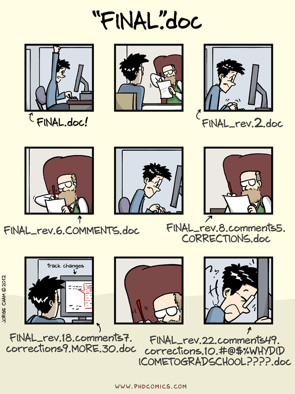
1. Introduction
In this episode, you will learn about the git version control system and how to use it in your R project from RStudio.
We will see how to trace edits and modifications made to your R Markdown document. Also, we will demonstrate how you can revert changes if needed or experiment safely with changes on your valuable code.
1.1 What is a version control system and why scientists should use it?
In the context of a research project, a version control system will help you to manage your project history, progress and support active collaboration with your colleagues but also with you (past, present and future self).
As a concrete example, this is something we might have all experienced in the past when keeping track of file versions:
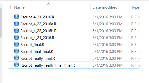
Version control is an essential tool in data analysis
Version control will help you to avoid this file nightmare but also fosters other good practices related to code.
1.2 Five reasons to use a version control system in research
- Tell the story: The history of your commit messages will describe your project progress.
- Travel back in time: a version control system makes it easy to compare different time points of your project smoothly. If you want to compare the stage of your project a year ago from now, it only takes one command-line of code.
- Experiment with changes: if you want to make changes in a script, you can first make a “snapshot” of the project status before experimenting with changes. As a researcher, this might be a second nature for you!
- Backup your work: by being able to linking your local repository (folder) to a distant online host, a version control system backs up your precious work instantly.
- Collaborate easily on projects: having a web-hosted synchronised version of your project will encourage collaboration with other researchers. Think about a colleague of yours being able to add a script to make a figure for your first PhD publication for instance.
There are possibly other important reasons why you could use a version control system for your research project. While originally created for software development, a common usage in scientific research is to track versions of datasets, scripts or figures easily and efficiently.
1.3 git is a popular version control software
![]()
One of the most used version control software out there is git. It is a cross-platform tool that is available on Mac and Linux OS natively and that needs to be installed on Windows check the Setup section on how to do this. git is a version control system primarily used in software development.
Definition
Defined simply:
gitis an application that runs on your computer like a web browser or a word processor (Tom Stuart).
1.4 Collaborating with yourself with git
Using your recently acquired flashy R skills, you are now ready to apply them to your scientific project You start by creating an R Markdown document, add code and text comments, generate an HTML report, save your R Markdown document, etc.
But how do you make sure that your changes are properly been saved and tracked? What is your backup strategy? This is where git will come in handy.
2. Tell the story of your project
Compare two solutions below, one without git and one with:
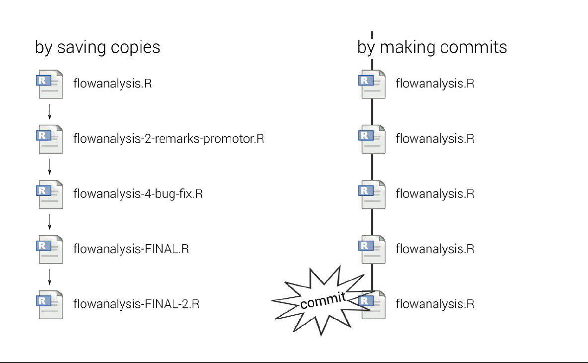
Discussion
Can you list the potential and proven drawbacks of keeping track of changes by saving copies of the files?
In the follow-up section, we will see how to tell a story about the changes applied to our R Markdown document. This storyline will be composed of the git commit messages.
Let’s see how we can use git powerful file versioning from within RStudio.
2.1 Create a new RStudio project
Projects in RStudio are a great feature and work very well in combination with git.
Go to RStudio and click on File > New Project > New directory.
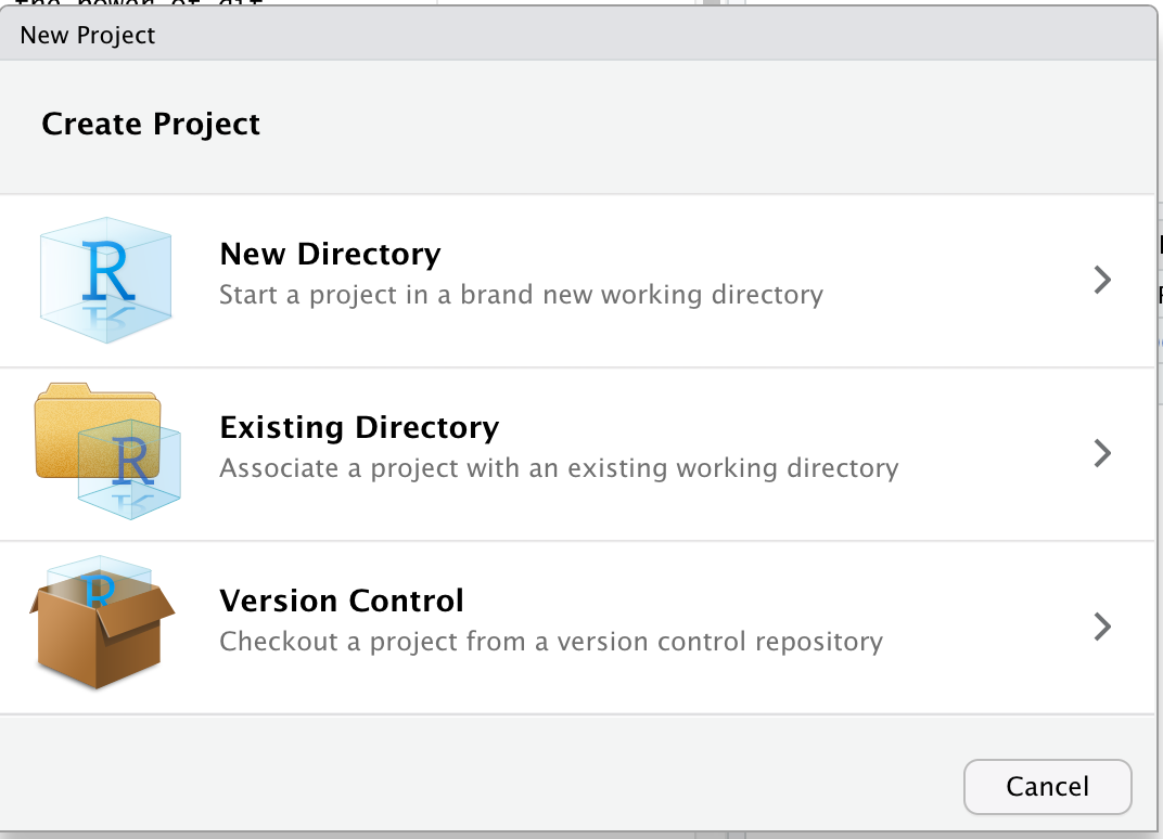
Then select New project
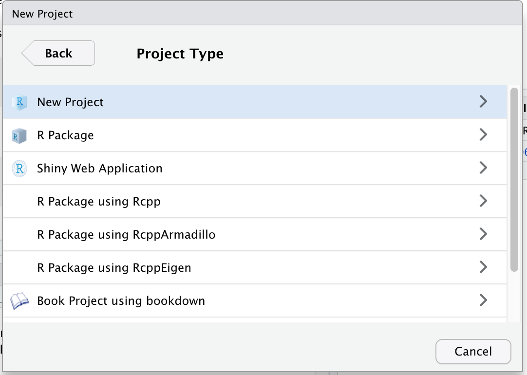
We will call our new project “learning_git”
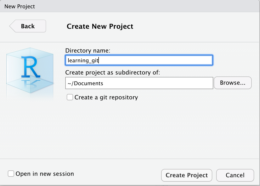
2.2 Create a new R Markdown document
Go to File > New File > R Markdown and call it “learning git”. Click “OK”. It should open this new R Markdown document.
Below the ## R Markdown, add a new code chunk, and copy this code:
library("tidyverse")
Save your document under the name learning_git.Rmd. You should see this in your File pane:
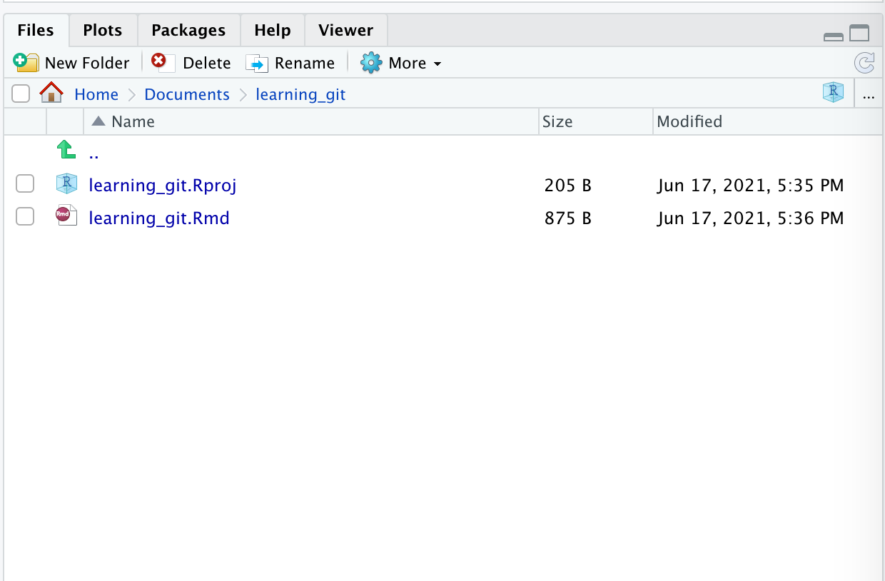
2.3 Initialize git from within the folder
Great, but git is still unaware of things that happen in this R project folder. Let’s change that.
In the console pane, click on “Terminal” to get access to a Shell from within RStudio. We will initialise git in this folder.
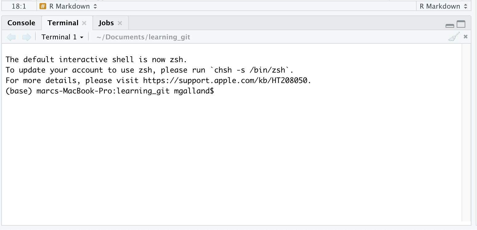
This is a regular Shell in which you can type any command-line instruction. Let’s type this:
git init
This command created a hidden folder called .git/ that will contain all information needed by git to recapitulate your file changes, project history, etc.
Try typing this:
ls -l .git/
This will show you what happened behing the hood:
(base) marcs-MacBook-Pro:learning_git mgalland$ ls -l .git/
total 24
-rw-r--r--   1 mgalland  staff   23 Jun 17 17:45 HEAD
-rw-r--r--   1 mgalland  staff  137 Jun 17 17:45 config
-rw-r--r--   1 mgalland  staff   73 Jun 17 17:45 description
drwxr-xr-x  14 mgalland  staff  448 Jun 17 17:45 hooks
drwxr-xr-x   3 mgalland  staff   96 Jun 17 17:45 info
drwxr-xr-x   4 mgalland  staff  128 Jun 17 17:45 objects
drwxr-xr-x   4 mgalland  staff  128 Jun 17 17:45 refs
2.4 Track file changes with git
Close and restart RStudio to show the “git” tab in the environment pane. You should see this:
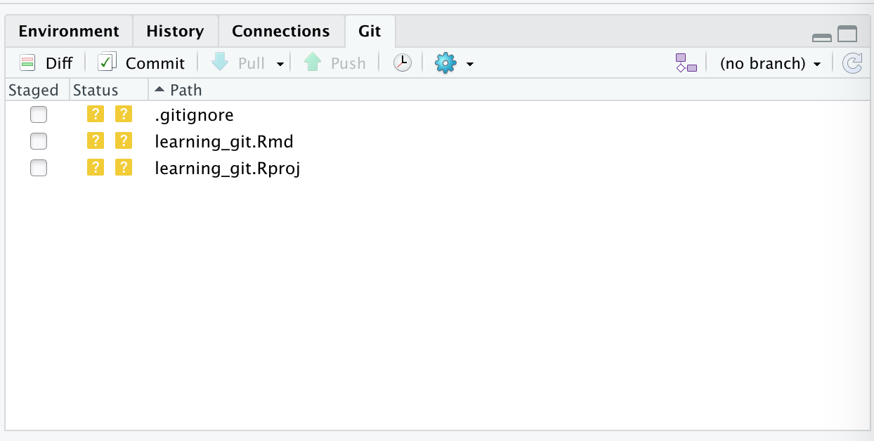
For now, git does not track anything in this RStudio project folder.
We would like git to track changes in our learning_git.Rmd document. To do this, click in the empty checkbox:
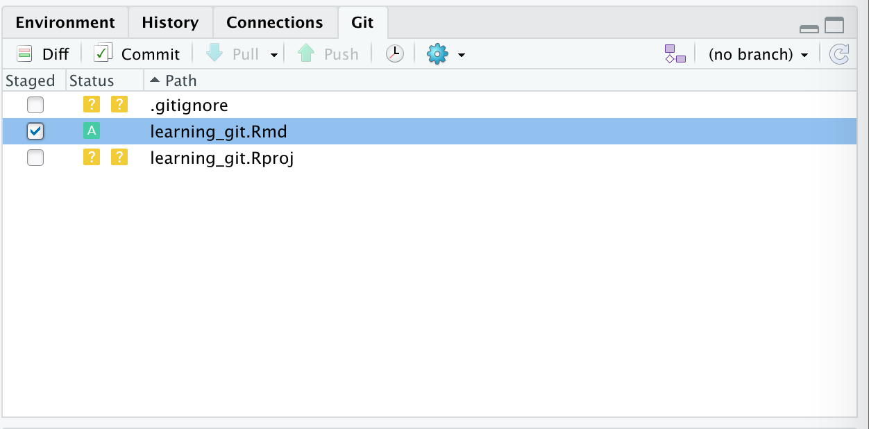
You can see that there is now a small green “A” next to the learning_git.Rmd file under the “Status” column. This means that our file is now being tracked by git.
2.5 Making changes and visualising them.
We will first:
- Import the
gapminderdataset. - Make a plot of the GDP per capita along the years for Canada.
- Write a small comment about the plot.
These 3 steps will all have their own commit message. Let’s start.
In your Rmd document, create a new code chunk and add this:
gapminder <- readr::read_csv('https://raw.githubusercontent.com/carpentries-incubator/open-science-with-r/gh-pages/data/gapminder.csv')
Save your learning_git.Rmd document
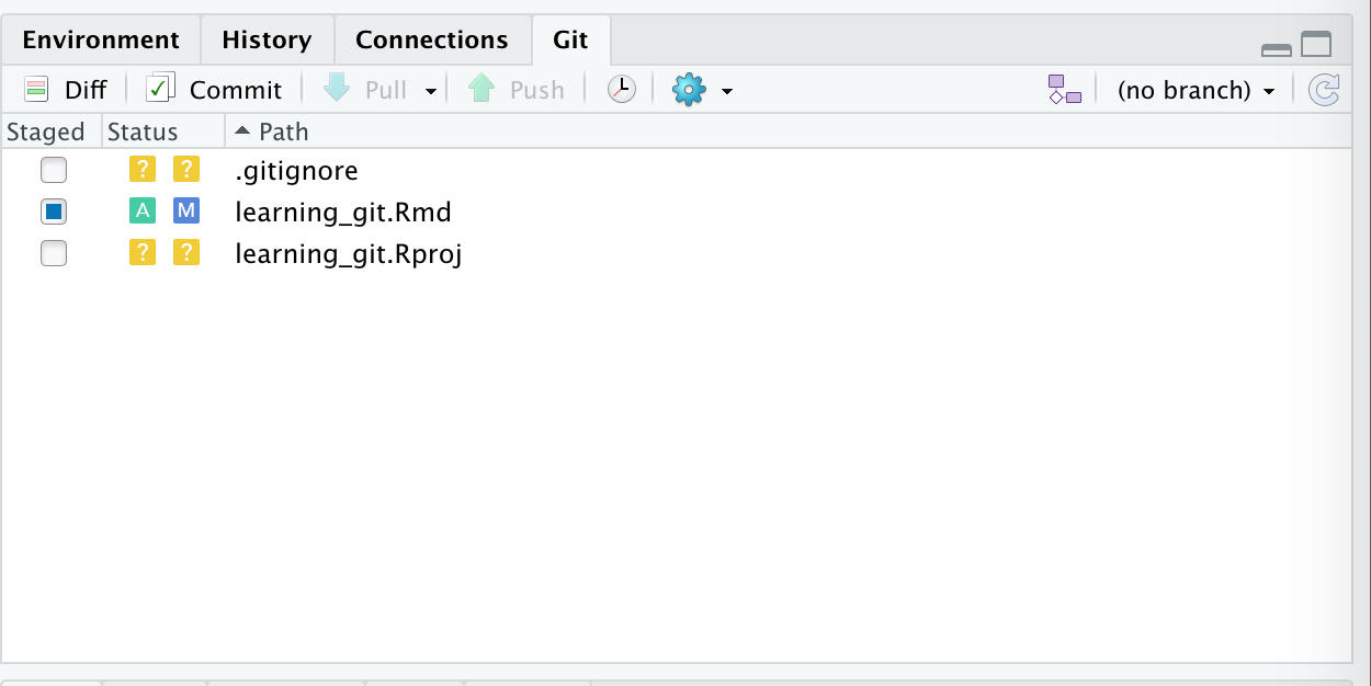
You see a small blue “M” button next to your learning_git.Rmd file. This stands for “Modified”. You can visualise the changes in your Rmd document by selecting “diff”:
![]()
This opens a new window where you can see that 3 lines where added (shown in green). These lines are the code chunk we’ve added where we read the gapminder dataset.
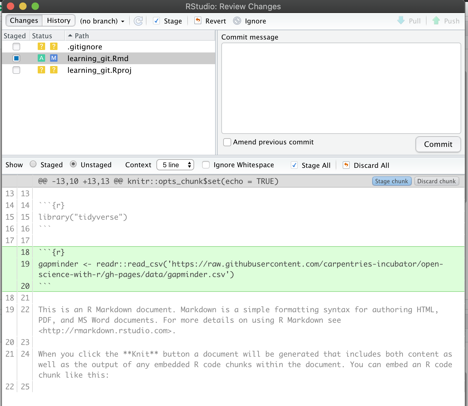
While we are in this “diff” view, we can write a small commit message to describe what happened to our document in a meaningful way.
In the “Commit message” write this little message:
Import the gapminder dataset

The gapminder dataset is imported using an online url.
It will be used to produce a plot of the GDP per year.
Now, click on commit. This will assign a unique identifier to your commit as git takes a snapshot of your learning_git.Rmd file.
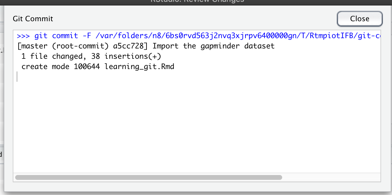
Let’s continue our work, add the changes and create commit messages.
Exercise
- Step 1: Add a scatterplot of the GDP per capita per year for Canada (use
geom_point). Save your Rmd document.- Step 2: Add the modifications by cliking the checkbox under “Staged” to see the blue “M” sign in RStudio git pane.
- Step 3: Click on “Diff” to open the new window where you should write a small commit message. Click on “Commit” when you’re done.
- Step 4: Write a small conclusion about the plot in your Rmd document.
- Step 5: save, add/stage changes, commit your changes with a small message.
If all went well, you can click on “History” to preview the history of commits that you have already made:
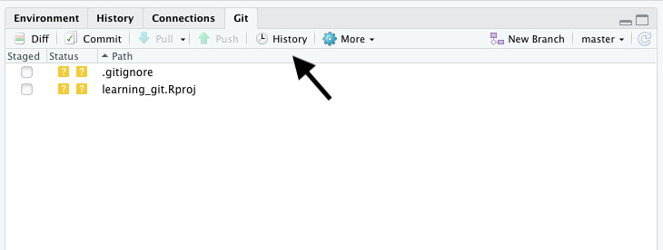
This gives you a history of your Rmd file and your project so far. These 3 commits are nicely placed on top of each other. Each of them has a unique SHA identifier to trace it back. We will see in the next section how to move back and forth in time using these SHA ids.
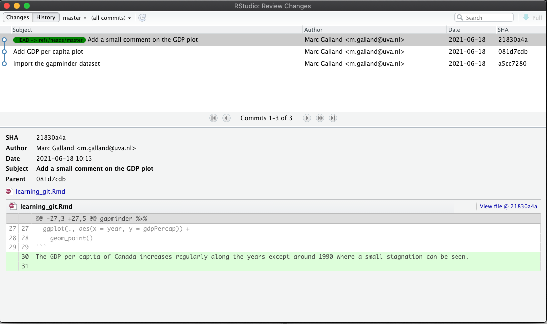
2.6 Great commits tell a great story
A good commit message
- Separate subject from body with a blank line
- Limit the subject line to 50 characters.
- Capitalize the subject line.
- Do not end the subject line with a period.
- Use the imperative mood in the subject line.
- Wrap the body at 72 characters.
- Use the body to explain what and why vs. how. The how is self-explainable from your code.
Here is an example of a good commit message:
Fix issue with dplyr filter function

By specifying the dplyr::filter() explicitely
avoid issues with other filter() functions
from other packages
3. Travel back in time

3.1 History of commits
If all went well in the previous exercise, you have 3 nicely self-explainable commits like this:
In this section we will see how to move back and forth between these commits safely. This can be useful to see what happened to a file or to revert to a previous commit (because you are not happy with the current version).
3.2 Back to the past
Imagine that you are not happy with your conclusion about the GDP per capita plot for Canada. Then, it would be useful to revert to a previous commit. In the history, we would like to revert to the previous commit with the message “Add GDP per capita plot”.
Go to the Terminal in the Console pane of RStudio and type:
git hist
This will output the commit history of your local folder where you are working.
* 21830a4 2021-06-18 | Add a small comment on the GDP plot (HEAD -> master) [Marc Galland]
* 081d7cd 2021-06-18 | Add GDP per capita plot [Marc Galland]
* a5cc728 2021-06-18 | Import the gapminder dataset [Marc Galland]
The commit id 21830a4 is the most recent one (also called the HEAD). The commit we would like to revert to has the commit identifier 081d7cd.
Important note
Your exact commit identifier should be different. Using
git histidentify your commit identifier that is required. Make sure you use your own commit identifier otherwise it will not work.
In git, the command to do this is called git checkout. In your terminal in RStudio, type:
git checkout 081d7cd
We get a lot of text messages.
Note: switching to '081d7cd'.

You are in 'detached HEAD' state. You can look around, make experimental
changes and commit them, and you can discard any commits you make in this
state without impacting any branches by switching back to a branch.

If you want to create a new branch to retain commits you create, you may
do so (now or later) by using -c with the switch command. Example:

  git switch -c <new-branch-name>

Or undo this operation with:

  git switch -

Turn off this advice by setting config variable advice.detachedHead to false

HEAD is now at 081d7cd Add GDP per capita plot
This simply tells us that our latest commit (the HEAD) is now pointing at the commit id 081d7cd where we added the GDP plot. Again you will have a different commit identifier and that’s totally normal.
Check your learning_git.Rmd file. It should have changed and the conclusion about the plot is now gone.
Actually not, git has just masked commits that were happening after the commit we checked out.
Question
Can you think about another way to delete the plot conclusion?
Solution
You can also delete the plot conclusion, save your Rmd document and commit this new change. Commits are as much about deleted code/text as about additions.
3.3 Back to the present
Ok, let’s get back to the latest commit in one step:
git checkout master
Now we retrieve our most up to date Rmd document.
4. Experiment with changes
One of the greatest feature of git is that it allows you to experiment with changes without any harm to your functional R script. Imagine that you want to change the way you perform statistics and see the consequences. This is easy with git.
4.1 Create a new branch
FIXME: create a branch called “barplot” where you modify the Canada GDP scatterplot into a bar plot.
4.2 Modify the plot
Modify your code that you previously wrote to make a bar plot instead of a scatterplot. Here is a suggestion:
gapminder %>%
  filter(country == "Canada") %>%
  ggplot(., aes(x = year, y = gdpPercap)) +
    geom_histogram(stat = "identity")
Make sure you add + commit your changes.
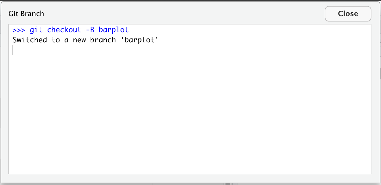
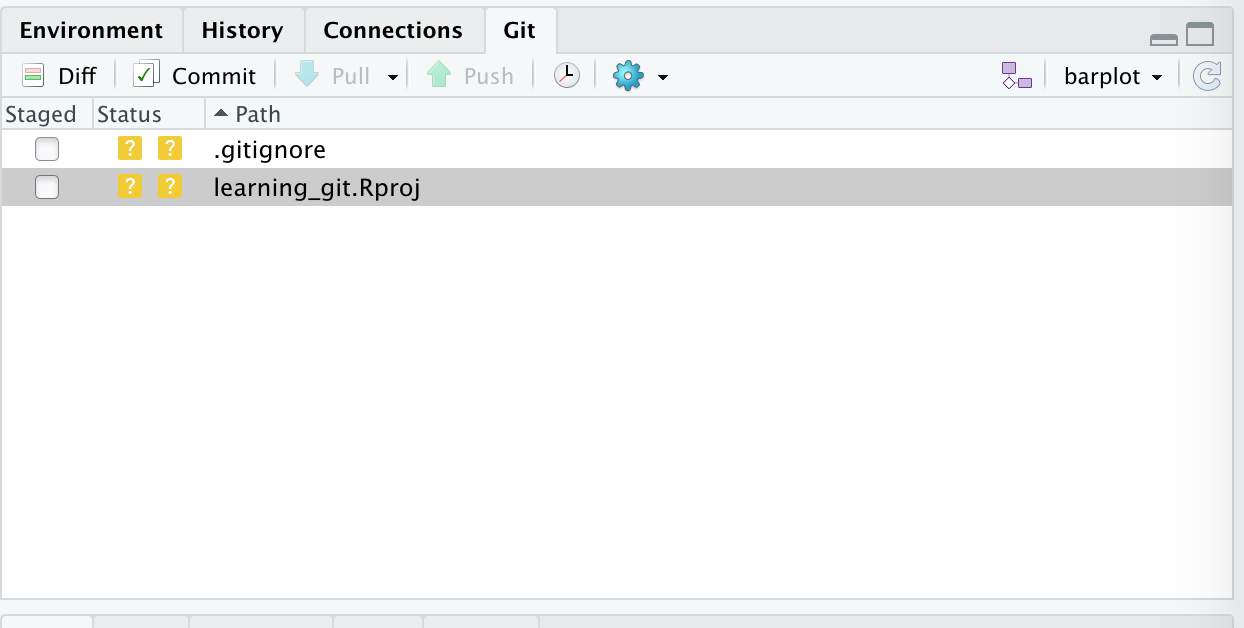
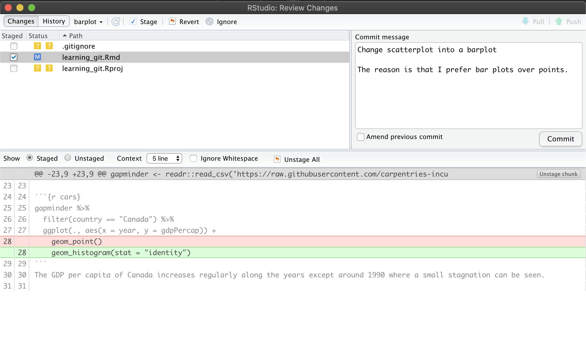
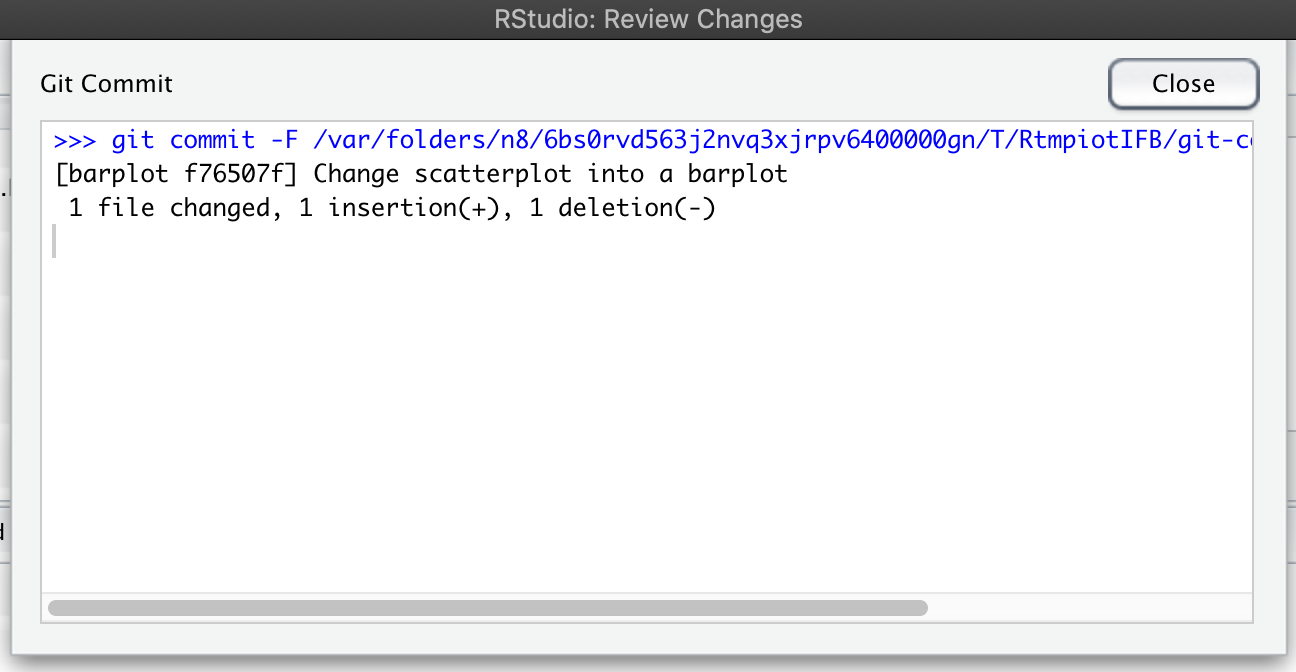
4.3 Switch back to the master branch
Once your changes are committed inside the barplot branch, you can easily switch back to the main branch called the master branch.
You can either use the branch tool in RStudio and select master or use the Terminal of RStudio (see below):
RStudio tool
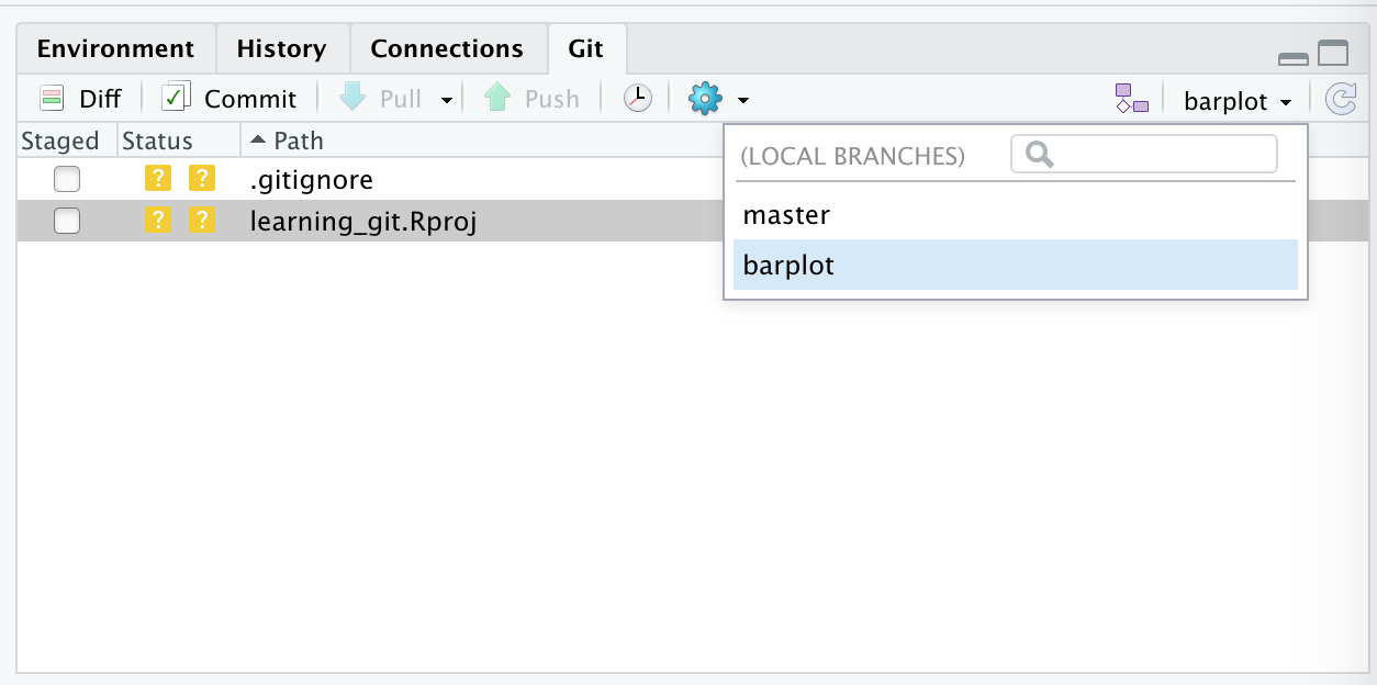
Terminal alternative
git checkout master
This will switch your Rmd document to its original content on the master branch. The plot is now a scatterplot.
Branch are key to
gitpowerBranches are a great feature since they allow you to experiment changes, test options without altering your main functional piece of work.
5. Recap of git commands
Before we dive in, there is a bit of technical terms to know.
| git command | description | RStudio equivalent |
|---|---|---|
git add |
asking git to track the file changes. This is also called “staging” the file. |  |
git commit |
taking a snapshot of the folder at a given time point. |  |
git status |
asking git to give an overview of changes to be committed, untracked files, etc. | None |
git hist |
list the history of commits |  |
git log |
showing the most recent commits. Do git log --oneline for more concision |
|
git checkout -b |
makes a new branch |  |
6. Resources
6.1 Links
- A “git for humans” presentation
- Jenny Bryan’s HappyGitWithR is very useful for troubleshooting, particularly the sections on Detect Git from RStudio and RStudio, Git, GitHub Hell (troubleshooting).
- Online game
- RStudio webinar on GitHub and RStudio
- Using git and GitHub for scientific writing
6.2 Troubleshooting
Sometimes, git integration with RStudio has issues.
- Issues with
gitand Mac OS X: https://github.com/jennybc/happy-git-with-r/issues/8
Key Points
In a version control system, file names do not reflect their versions.
gitacts as a time machine for files in a given repository under version control.
gitallows you to test changes and discard them if not relevant.A new RStudio project can be smoothly integrated with
gitto allow you to version control scripts and other files.
Collaborating with you and others with Github
Overview
Teaching: 30 min
Exercises: 30 minQuestions
How can I develop and collaborate on code with me or another scientist?
How can I give access to my code to another collaborator?
How can I keep code synchronised with another scientist?
How can I solve conflicts that arise from that collaboration?
What is Github?
Objectives
Be able to create a new repository and share it with another scientist.
Be able to work together on a R script through RStudio and Github integration.
Understand how to make issues and explore the history of a repository.
Table of contents
- 1. Introduction
- 2. Me, myself and GitHub
- 3. Collaborating with others
- 4. Merge conflicts
- 5. Explore on GitHub.com
- 6. Resources and credits
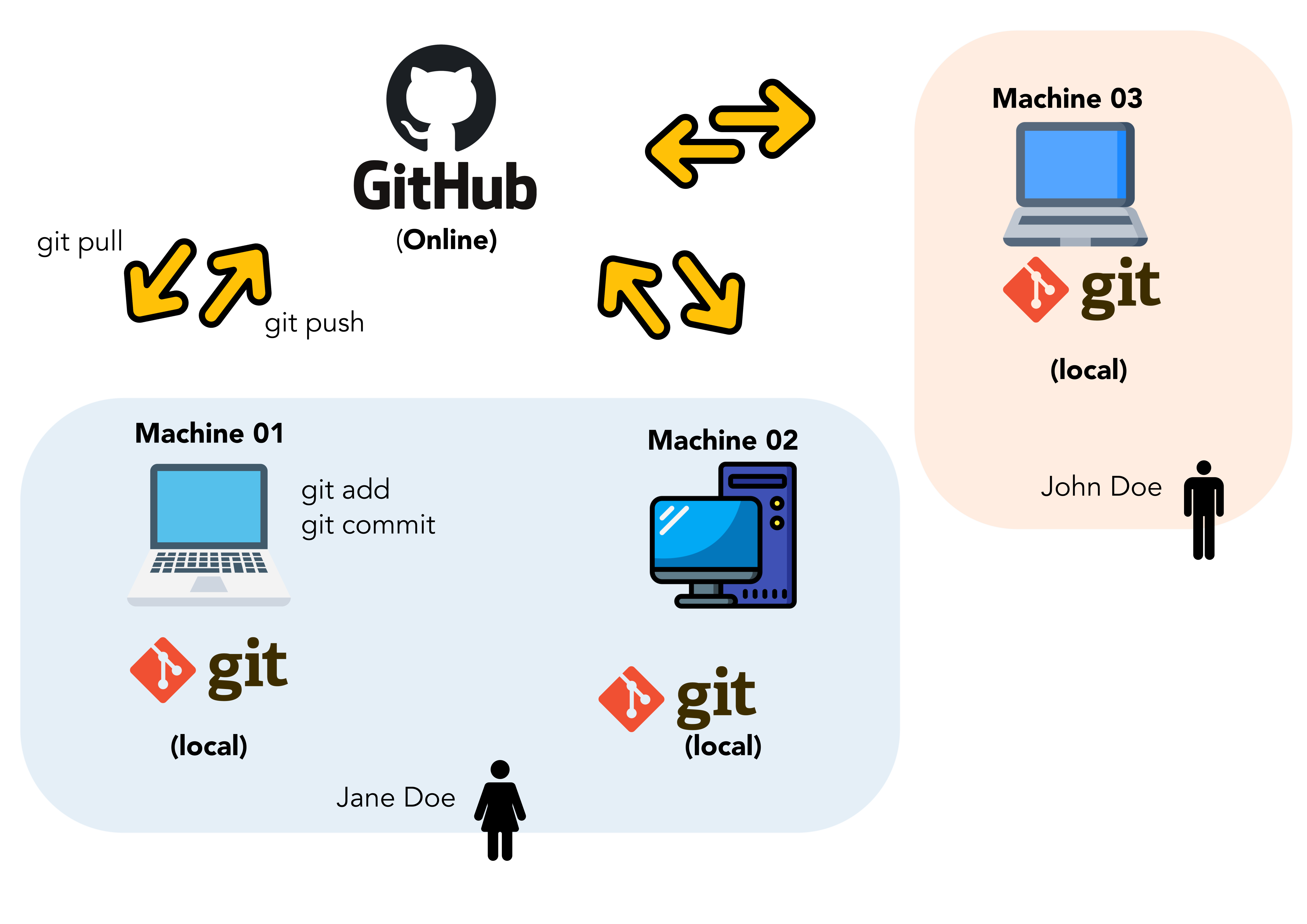
1. Introduction
In this episode, we will see different ways to collaborate using git and GitHub.
1.1 What is GitHub?
GitHub is a company recently acquired by Microsoft in 2018 that serves as a hosting service for code used in software development. It natively supports version control and interplays smoothly with local version control system like git.
Functionalities of GitHub includes:
- issues: report a bug, suggest code improvements, etc.
- access control: code can be made private or public, collaborators can be allowed access to certain repositories but not others, etc.
- service integration: GitHub allows you to trigger actions on other websites. For instance, when you make a release of your code, it can be automatically archived on Zenodo with a persistent identifier (doi).
- contributions: visualisation of contributions on code from different authors is easy and can be visualised at a glance.
1.2 GitHub jargon
Here is a small recap of GitHub technical terms you might encounter. Some are common with git so you could be familiar with some terms.
| GitHub jargon | human translation |
|---|---|
| user | a Github account for you (e.g., jules32). |
| organization | the Github account for one or more user (e.g., datacarpentry). |
| repository | a folder within the organization that includes files dedicated to a project. |
| commit | a snapshot of your project at a give time. Gets a unique commit identifier. |
| clone | process of making a local copy of a remote Github repository. This only needs to be done once (unless you mess up your local copy). |
| pull | copy changes on the remote Github repository to your local Github repository. This is useful if multiple people are making changes to a repository. |
| push | save local changes to remote Github |
1.3 GitHub fosters collaboration between you and yourself
Take a look at the scheme above. You can see that GitHub is used by Jane Doe to collaborate with herself between her two different computers, a laptop called machine 01 and a personal computer called machine 02. She uses git locally to keep track of her files and push her local changes online to the GitHub website.
In that sense, GitHub for her acts as a remote backup for her code, small datasets and perhaps everything related to her scientific work. Think about your next publication for instance.
1.4 GitHub supports collaboration with others
Of course, you might also want to collaborate with other scientists, perhaps a skilled statistician that could take a look at your data analysis or an R expert that could turn some piece of messy code into a magic function.
This is where GitHub becomes a sort of social network for scientific programmers. You can invite other researchers in your organization, create private repositories etc.
For instance, you can create a GitHub organization for your research group where all researchers would place their computational work.
GitHub acts as a manually synchronised dropbox for your files and project history. It allows you to visualize online your files, the commits you’ve made and the differences between your file versions.
2. Me, myself and GitHub
2.1 Setup
Checklist
You should have:
- a free GitHub account.
- You’ve installed
git.- You’ve introduced yourself to
gitin the previous episode.
In the previous episode, you have created an RStudio project called “learning_git”. In this section, we will connect this local project, under local version control with git, to a remote “folder” on GitHub.
2.2 Create a repository on GitHub
Step 1: Go to your personal GitHub account on GitHub.
Step 2: Click on “New” and name this new repository “me_and_myself”
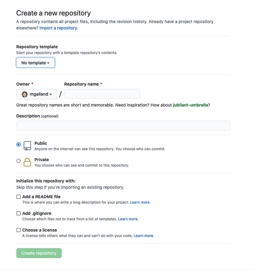
Add the required information, give a small description to your new repository, add a .gitignore file to ignore unnecessary files and add a license.
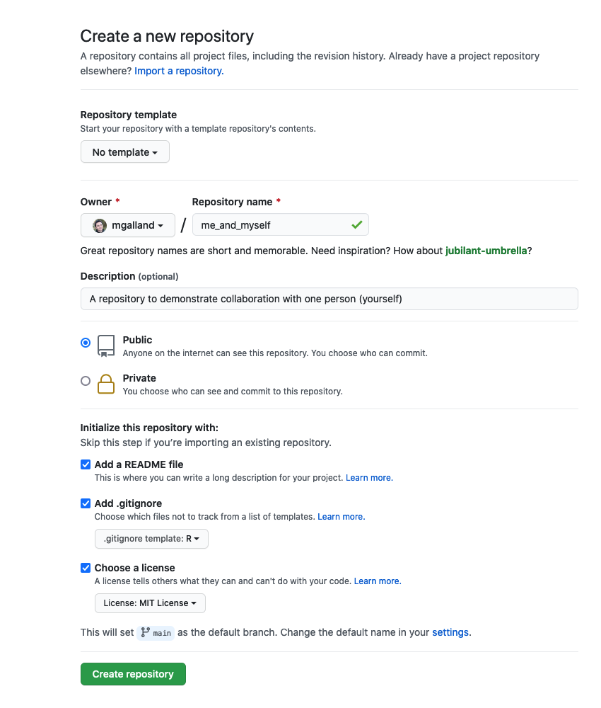
You can now see your new repository with a LICENSE, a .gitignore file and a README.md file.
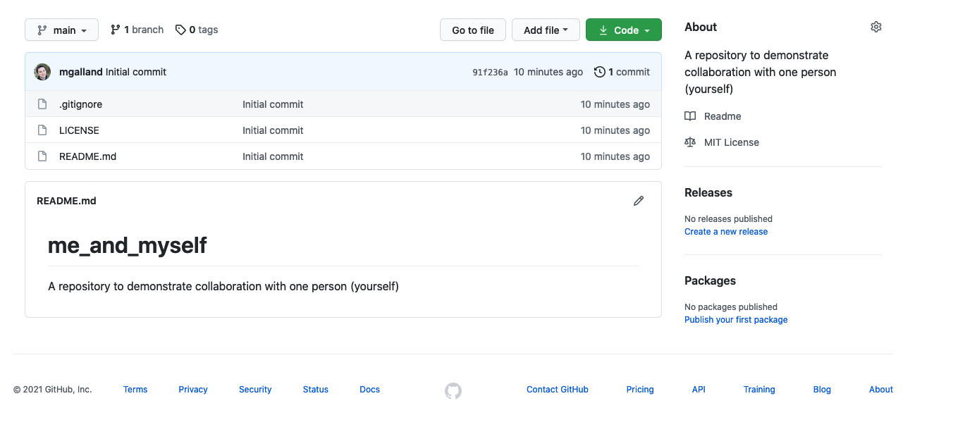
We are now going to clone this GitHub repository on our local computer from RStudio.
2.3 Create an RStudio project and clone this repository
Go to RStudio and click on File > New Project
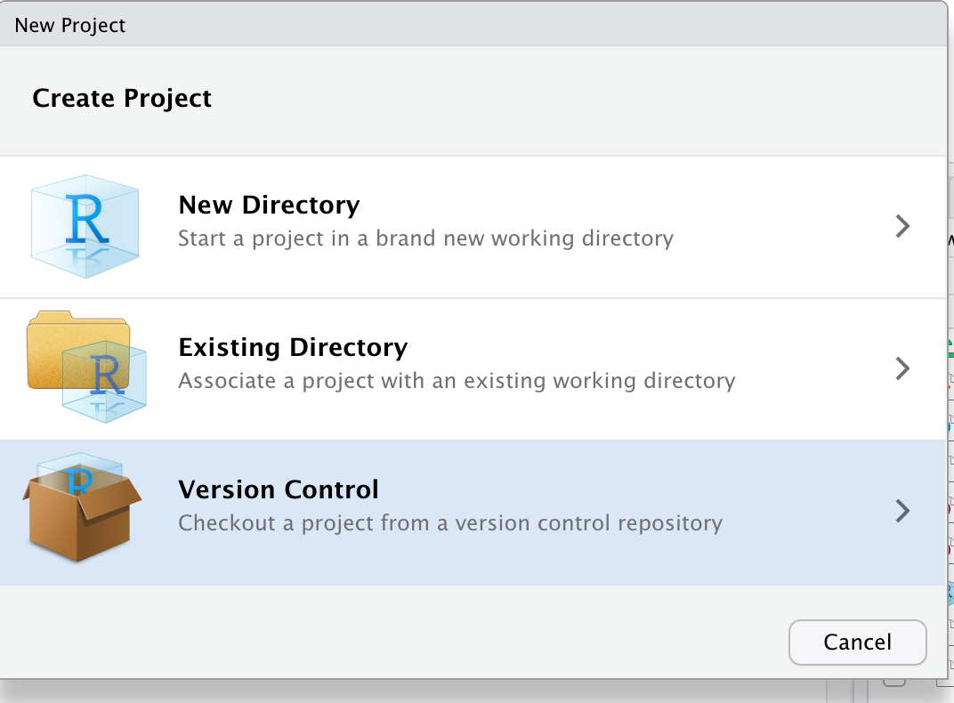
You are being asked to choose one version control system. Choose “git”:
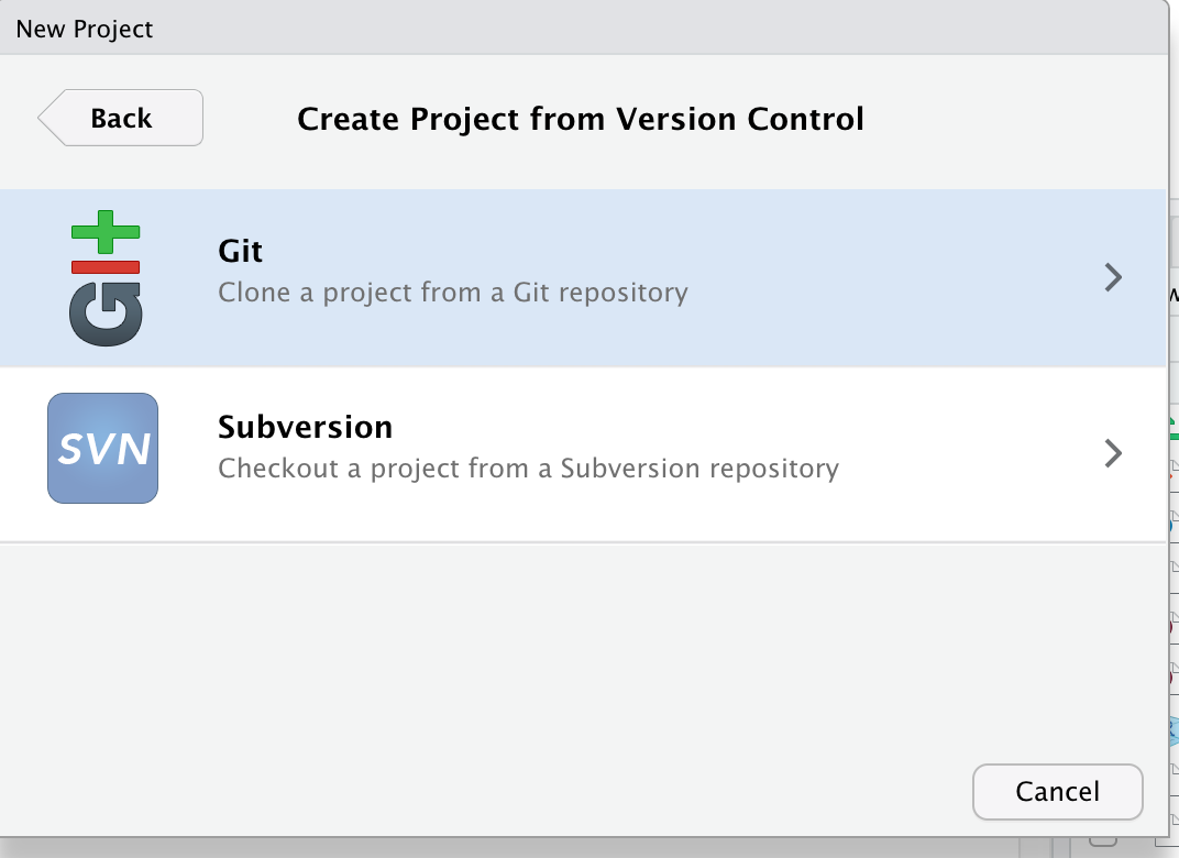
Finally, you can indicate from which remote repository you should start this new project. Go back online and copy-paste the link to your online repository.
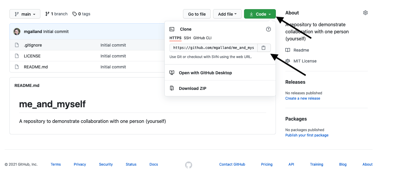
Finally, copy this information back in RStudio:
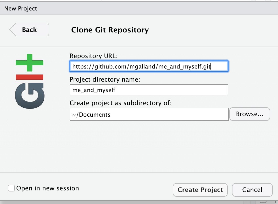
Your project is now ready to be imported from GitHub. If you do this, your local git and RStudio will be automatically configurated to work smoothly with the GitHub remote.
2.4 Practice
Exercise
Using your recently acquired RStudio, dplyr and
gitknowledge, perform the following steps:
- Step 1: create a new R Markdown document and name it “gapminder.Rmd”.
- Step 2: add two code chunks. In the first one, import the tidy gapminder dataset. In the second one, create a plot of the GDP per year for your favorite country.
gapminder <- readr::read_csv('https://raw.githubusercontent.com/carpentries-incubator/open-science-with-r/gh-pages/data/gapminder.csv')
- Step 3: save your “gapminder.Rmd” file.
- Step 4: using RStudio, stage your changes to that file, make a commit with a message.
- Step 5: push your changes online to GitHub.
- Step 6: go online to GitHub and see if you can retrieve your commit.
Your RStudio session should look like this. See the green “A” button that shows that your file has been brought to git attention.
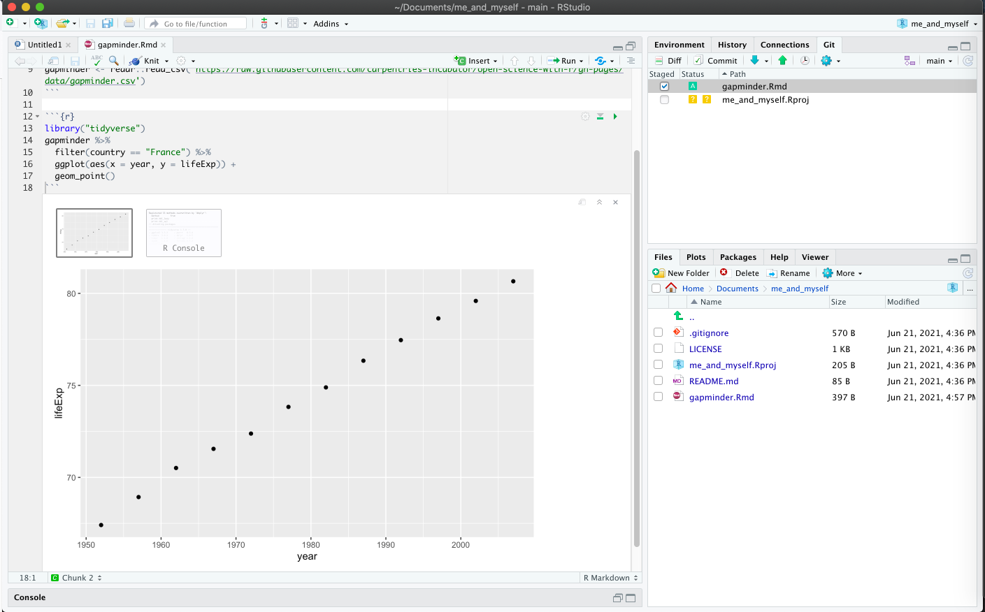
You should have made a commit message like this:
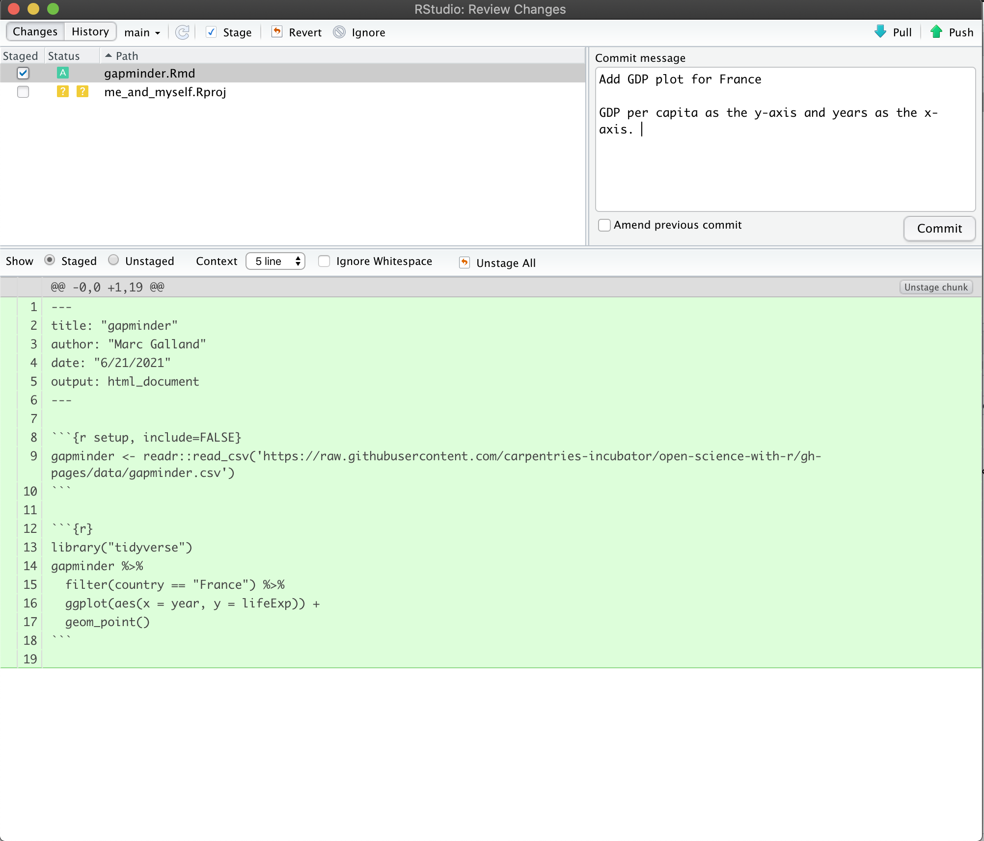
Finally click on “push” to update the GitHub online remote.
Question
Can you find the commit id in your GitHub repository?
Looking closely online, you see the commit identifier next to its time.
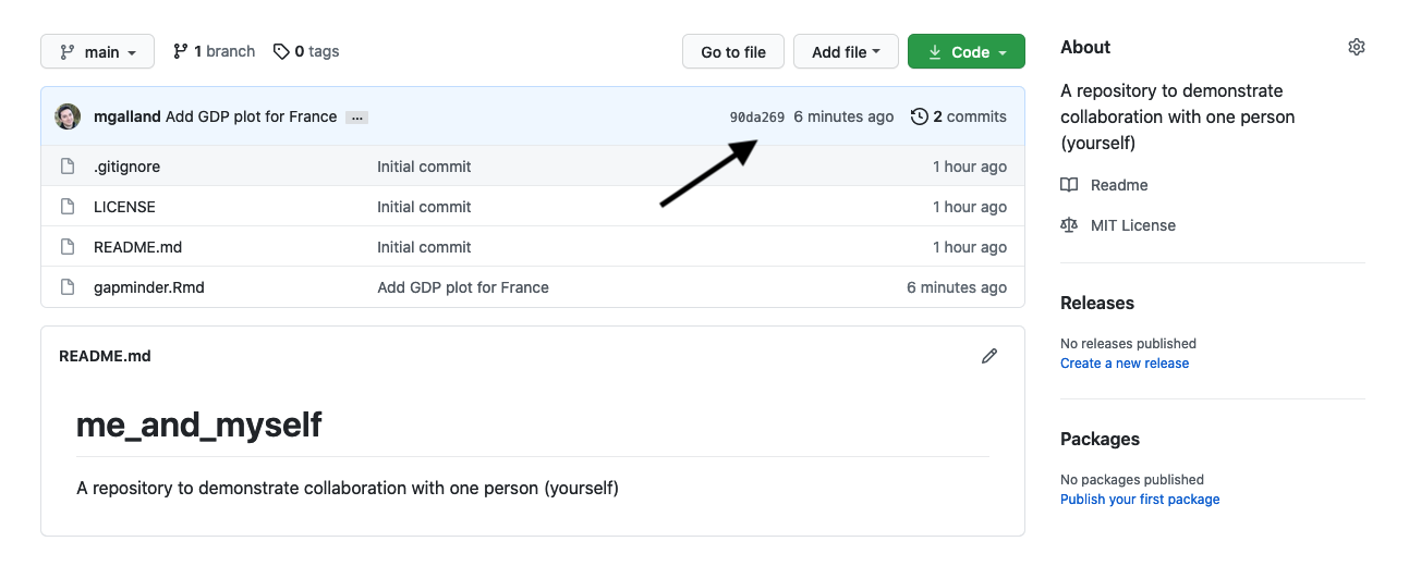
3. Collaborating with others
The collaborative power of GitHub and RStudio is really game changing. So far we’ve been collaborating with our most important collaborator: ourselves. But, we are lucky that in science we have so many other collaborators, so let’s learn how to accelerate our collaborations with them through GitHub.
We are going to teach you the simplest way to collaborate with someone, which is for both of you to have privileges to edit and add files to a repository. GitHub is built for software developer teams but we believe that it can also be beneficial to scientists.
We will do this all with a partner, and we’ll walk through some things all together, and then give you a chance to work with your collaborator on your own.
3.1 Pair up and work collaboratively
- Make groups of two scientists. They will collaborate through Github.
- Decide who will own the Github repository: this will be the “owner” also referred to as Partner 1.
- The other scientist will be called the “collaborator” also referred to as Partner 2.
- Please write your role on a sticky note and place it on your laptop to remember who you are!
3.2 Owner (Partner 1) setup
3.2.1 Create a Github repository
The repository “owner” will connect to Github and create a repository called first-collaboration. We will do this in the same way that we did in the “Version control with git and Github” episode.
3.2.2 Create a gh-pages branch
We aren’t going to talk about branches very much, but they are a powerful feature of git and GitHub. I think of it as creating a copy of your work that becomes a parallel universe that you can modify safely because it’s not affecting your original work. And then you can choose to merge the universes back together if and when you want.
By default, when you create a new repo you begin with one branch, and it is named master. When you create new branches, you can name them whatever you want. However, if you name one gh-pages (all lowercase, with a - and no spaces), this will let you create a website. And that’s our plan. So, owner/partner 1, please do this to create a gh-pages branch:
On the homepage for your repo on GitHub.com, click the button that says “Branch:master”. Here, you can switch to another branch (right now there aren’t any others besides master), or create one by typing a new name.
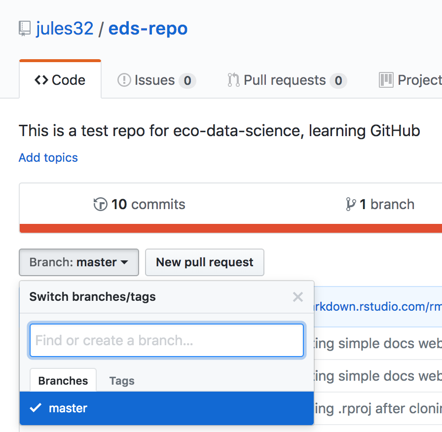
Let’s type gh-pages.
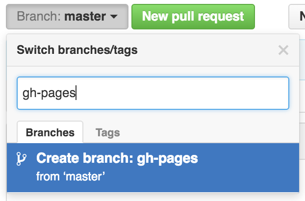
Let’s also change gh-pages to the default branch and delete the master branch: this will be a one-time-only thing that we do here:
First click to control branches:
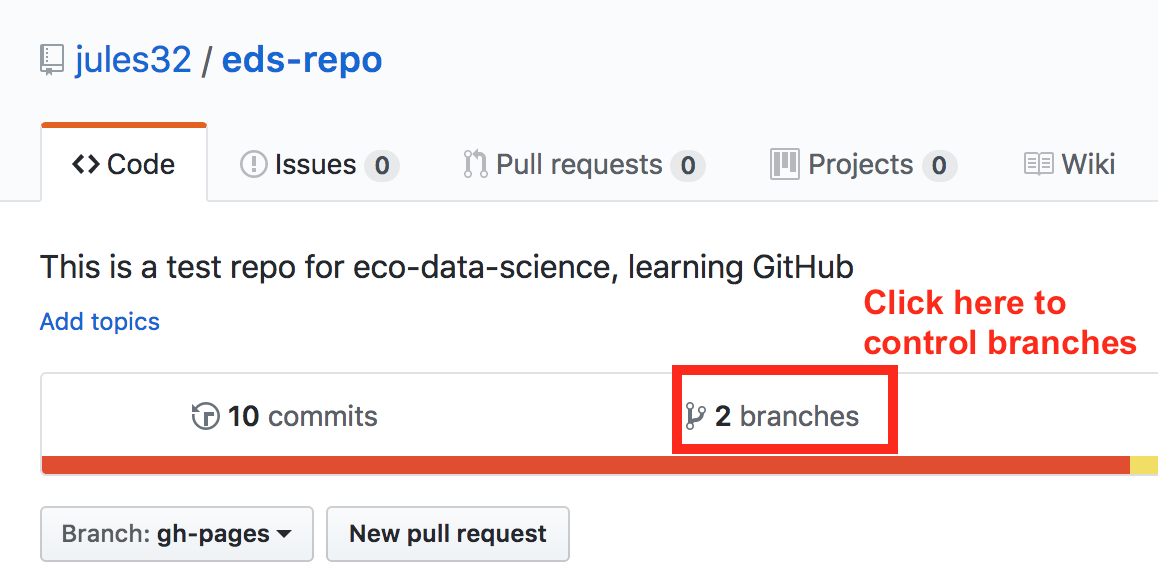
And then click to change the default branch to gh-pages. I like to then delete the master branch when it has the little red trash can next to it. It will make you confirm that you really want to delete it, which I do!
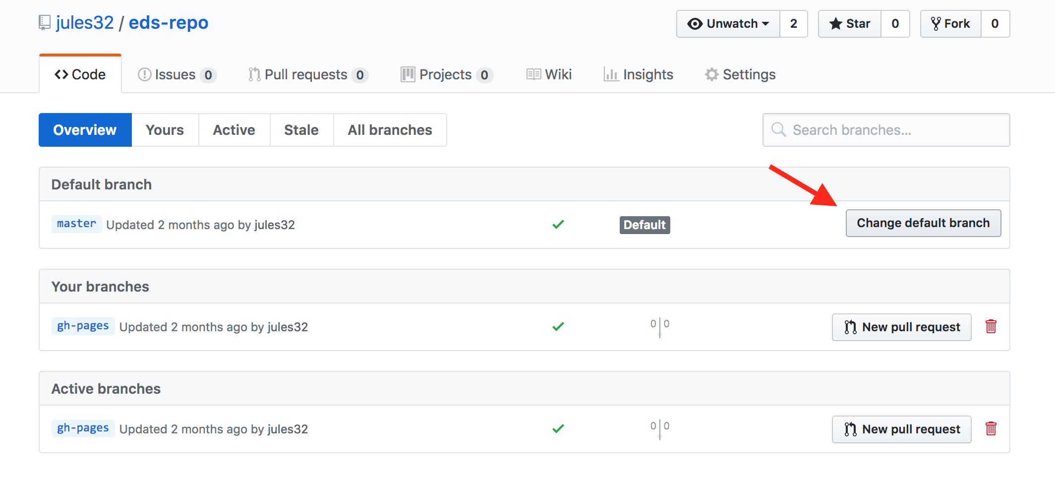
3.3 Give your collaborator administration privileges (Partner 1 and 2)
Now, Partner 1, go into Settings > Collaborators > enter Partner 2’s (your collaborator’s) username.
Partner 2 then needs to check their email and accept as a collaborator. Notice that your collaborator has “Push access to the repository” (highlighted below):
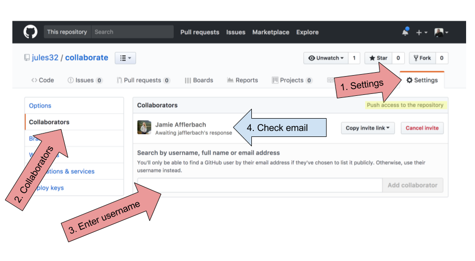
3.4 Clone to a new Rproject (Owner Partner 1)
Now let’s have Partner 1 clone the repository to their local computer. We’ll do this through RStudio like we did before (see the “Version control with git and Github:Clone your repository using RStudio” episode section. But, we’ll do this with a final additional step before hitting the “Create Project”: we will select “Open in a new Session”.
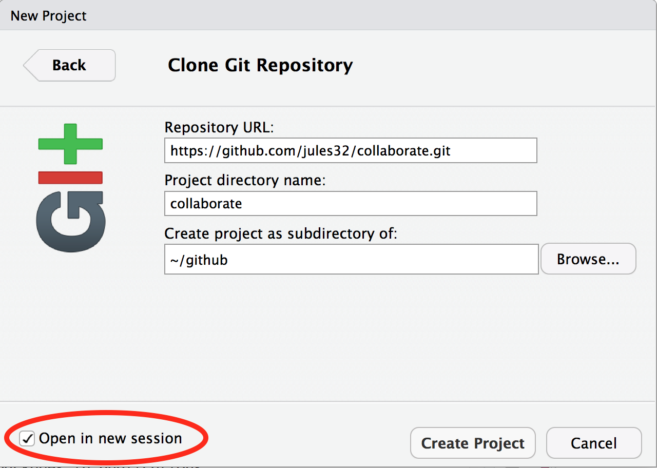
Opening this Project in a new Session opens up a new world of awesomeness from RStudio. Having different RStudio project sessions allows you to keep your work separate and organized. So you can collaborate with this collaborator on this repository while also working on your other repository from this morning. I tend to have a lot of projects going at one time:
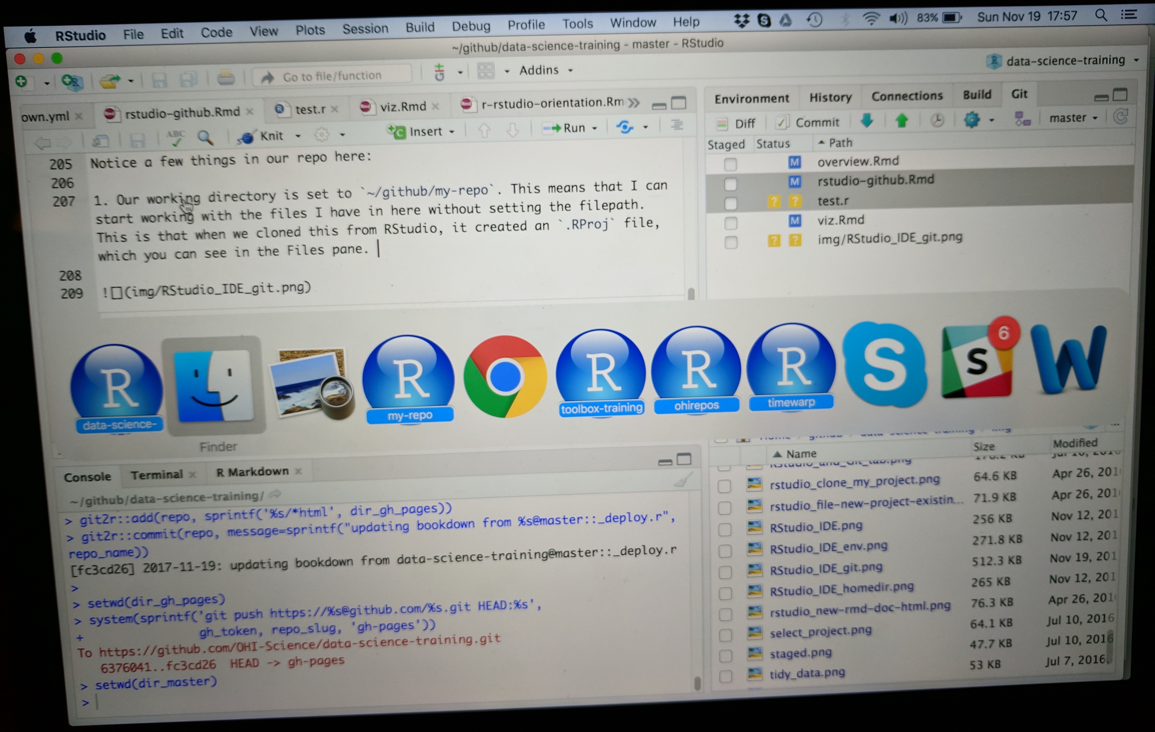
Have a look in your git tab.
Like we saw earlier, when you first clone a repo through RStudio, RStudio will add an .Rproj file to your repo. And if you didn’t add a .gitignore file when you originally created the repo on GitHub.com, RStudio will also add this for you. So, Partner 1, let’s go ahead and sync this back to GitHub.com.
Remember:
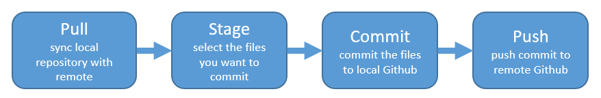
Let’s confirm that this was synced by looking at GitHub.com again. You may have to refresh the page, but you should see this commit where you added the .Rproj file.
3.5 Collaborator (Partner 2) part
3.5.1 Clone to a new Rproject (Partner 2)
Now it’s Partner 2’s turn! Partner 2, clone this repository following the same steps that Partner 1 just did. When you clone it, RStudio should not create any new files — why? Partner 1 already created and pushed the .Rproj and .gitignore files so they already exist in the repo.
Discussion point
Question: When you clone it, RStudio should not create any new files — why?
Solution
Partner 1 already created and pushed the
.Rprojand.gitignorefiles so they already exist in the repo.
3.5.2 Edit a file and sync (Partner 2)
Let’s have Partner 2 add some information to the README.md. Let’s have them write:
Collaborators:

- Partner 2's name
When we save the README.md, And now let’s sync back to GitHub.
When we inspect on GitHub.com, click to view all the commits, you’ll see commits logged from both Partner 1 and 2!
Discussion point
Questions:
- Would you be able to clone a repository that you are not a collaborator on?
- What do you think would happen? Try it!
- Can you sync back?
Solution
- Yes, you can clone a repository that is publicly available.
- If you try to clone it on your local machine, it does work.
- Unfortunately, if you don’t have write permissions, you cannot contribute. You would have to ask for write/push writes.
3.6 State of the Repository
OK, so where do things stand right now? GitHub.com has the most recent versions of all the repository’s files. Partner 2 also has these most recent versions locally. How about Partner 1?
Partner 1 does not have the most recent versions of everything on their computer!.
Discussion point
Question: How can we change that? Or how could we even check?
Solution
Use the
pullcommand to update your local version of the remote repository.
Let’s have Partner 1 go back to RStudio and Pull. If their files aren’t up-to-date, this will pull the most recent versions to their local computer. And if they already did have the most recent versions? Well, pulling doesn’t cost anything (other than an internet connection), so if everything is up-to-date, pulling is fine too.
I recommend pulling every time you come back to a collaborative repository. Whether you haven’t opened RStudio in a month or you’ve just been away for a lunch break, pull. It might not be necessary, but it can save a lot of heartache later.
4. Merge conflicts
What kind of heartache are we talking about? Let’s explore.
Stop and watch: demo time
Stop and watch me create and solve a merge conflict with my Partner 2, and then you will have time to recreate this with your partner.
4.1 Demo
Within a file, GitHub tracks changes line-by-line. So you can also have collaborators working on different lines within the same file and GitHub will be able to weave those changes into each other – that’s it’s job! It’s when you have collaborators working on the same lines within the same file that you can have merge conflicts. Merge conflicts can be frustrating, but they are actually trying to help you (kind of like R’s error messages). They occur when GitHub can’t make a decision about what should be on a particular line and needs a human (you) to decide. And this is good – you don’t want GitHub to decide for you, it’s important that you make that decision.
Me = partner 1. My co-instructor = partner 2.
Here’s what me and my collaborator are going to do:
- My collaborator and me are first going to pull.
- Then, my collaborator and me navigate to the README file within RStudio.
- My collaborator and me are going to write something in the same file on the same line. We are going to write something in the README file on line 7: for instance, “I prefer R” and “I prefer Python”.
- Save the README file.
- My collaborator is going to pull, stage, commit and push.
- When my collaborator is done, I am going to pull.
- Error! Merge conflict!
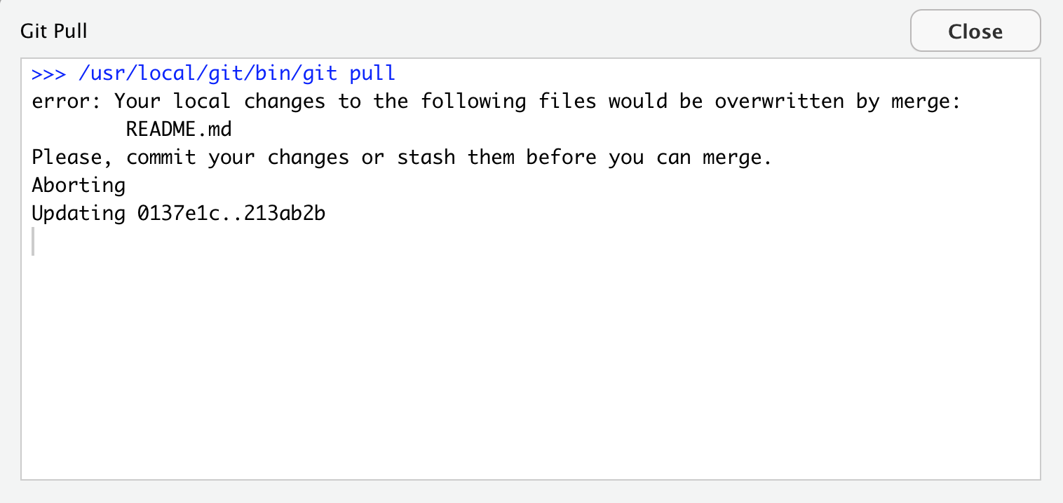
I am not allowed to to pull since GitHub is protecting me because if I did successfully pull, my work would be overwritten by whatever my collaborator had written.
GitHub is going to make a human (me in this case) decide. GitHub says, “either commit this work first, or stash it”. Stashing means “ (“save a copy of the README in another folder somewhere outside of this GitHub repository”).
Let’s follow their advice and have me to commit first. Great. Now let’s pull again.
Still not happy!
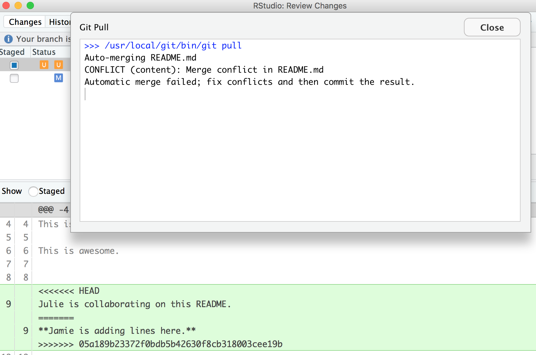
OK, actually, we’re just moving along this same problem that we know that we’ve created: Both me and my collaborator have both added new information to the same line. You can see that the pop-up box is saying that there is a CONFLICT and the merge has not happened. OK. We can close that window and inspect.
Notice that in the git tab, there are orange Us; this means that there is an unresolved conflict, and it is not staged with a check anymore because modifications have occurred to the file since it has been staged.
Let’s look at the README file itself. We got a preview in the diff pane that there is some new text going on in our README file:
<<<<<<< HEAD
Julie is collaborating on this README.
=======
**Jamie is adding lines here.**
>>>>>>> 05a189b23372f0bdb5b42630f8cb318003cee19b
In this example, I am Jamie and my collaborator is Julie. GitHub is displaying the line that Julie wrote and the line Jamie wrote separated by =======. So these are the two choices that Partner 2 has to decide between, which one do you want to keep? Where where does this decision start and end? The lines are bounded by <<<<<<<HEAD and >>>>>>>long commit identifier.
So, to resolve this merge conflict, my collaborator has to chose, and delete everything except the line they want. So, they will delete the <<<<<<HEAD, =====, >>>>long commit identifier and one of the lines that they don’t want to keep.
Do that, and let’s try again. In this example, we’ve kept my (Jamie’s) line:
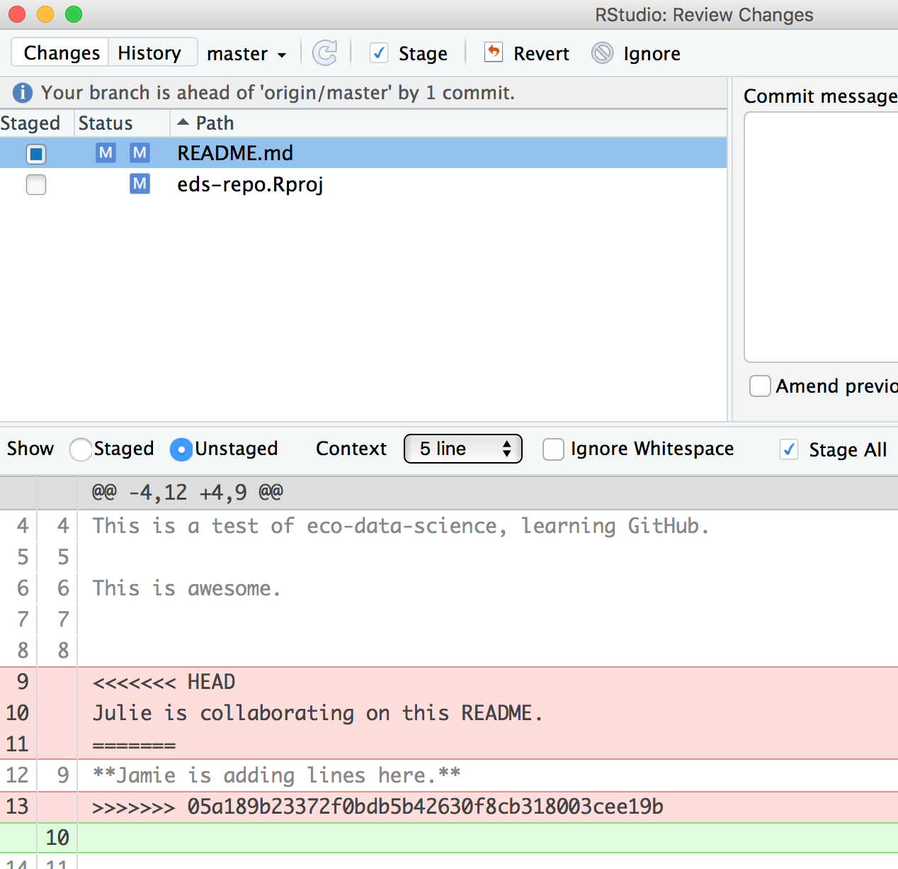
Then be I need to stage and write a commit message. I often write “resolving merge conflict” or something so I know what I was up to. When I stage the file, notice how now my edits look like a simple line replacement (compare with the image above before it was re-staged):
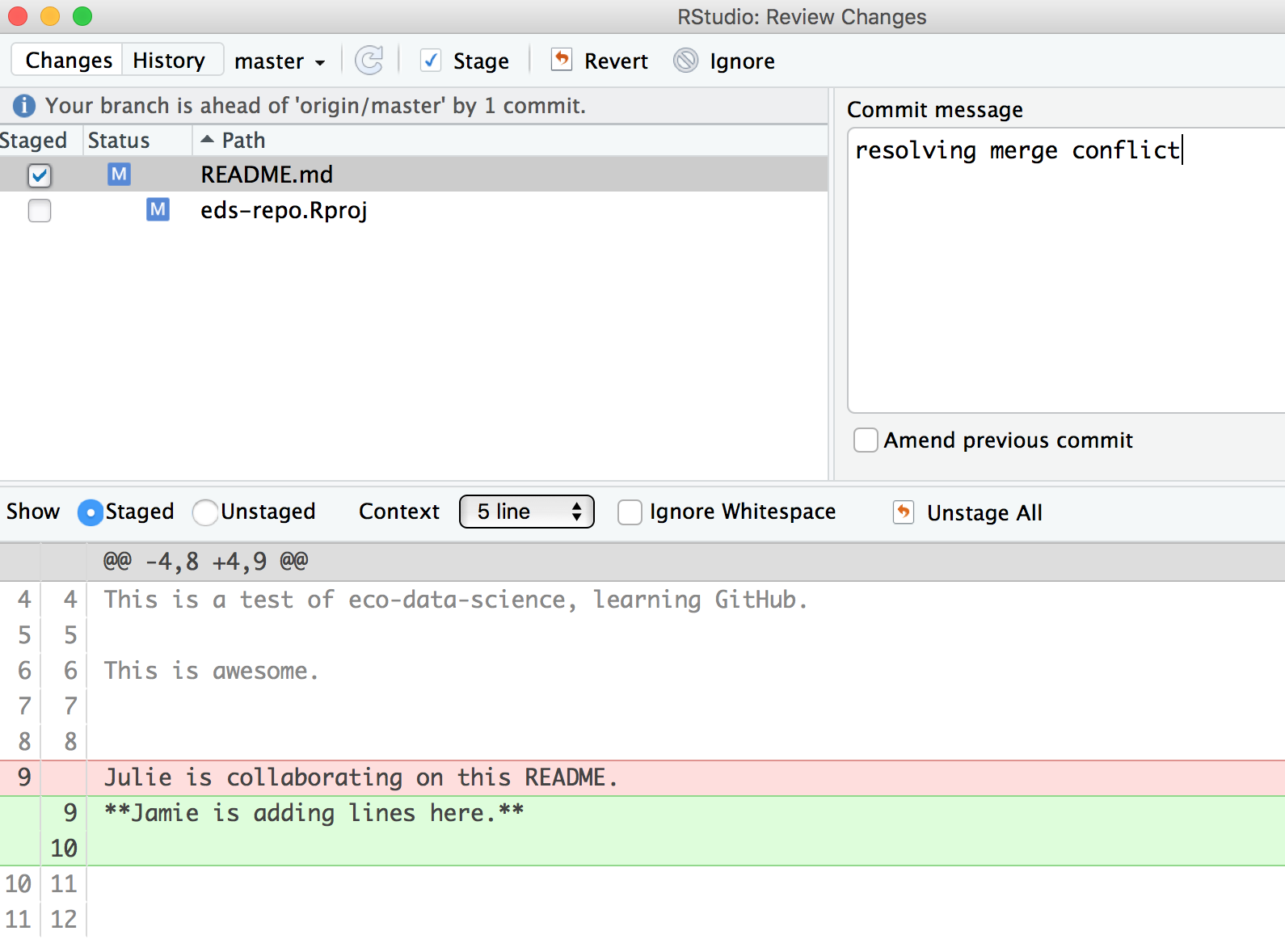
4.2 Your turn
Exercise
- Create a merge conflict with your partner, like we did in the example above.
- Try to fix it.
- Try other ways to get and solve merge conflicts. For example, when you get the following error message, try both ways (commit or stash. Stash means copy/move it somewhere else, for example, on your Desktop temporarily).
4.3 Avoiding merge conflicts
One way to avoid merge conflicts is to pull often, commit and push often.
Also, talk with your collaborators. Even on a very collaborative project (e.g. a scientific publication), you are actually rarely working on the exact same file at any given time. And if you are, make sure you talk in-person or through chat applications (Slack, Gitter, Whatsapp, etc.).
But merge conflicts will occur and some of them will be heartbreaking and demoralizing. They happen to me when I collaborate with myself between my work computer and laptop. So protect yourself by pulling and syncing often!
4.4 Create your collaborative website
OK. Let’s have Partner 2 create a new RMarkdown file. Here’s what they will do:
- Pull!
- Create a new RMarkdown file and name it
index.Rmd. Make sure it’s all lowercase, and namedindex.Rmd. This will be the homepage for our website! - Maybe change the title inside the Rmd, call it “Our website”
- Knit!
- Save and sync your .Rmd and your .html files: pull, stage, commit, pull, push.
- Go to GitHub.com and go to your rendered website! Where is it? Figure out your website’s url from your github repo’s url. For example:
- my github repo: https://github.com/jules32/collab-research
- my website url: https://jules32.github.io/collab-research/
- note that the url starts with my username.github.io
So cool! On websites, if something is called index.html, that defaults to the home page. So https://jules32.github.io/collab-research/ is the same as https://jules32.github.io/collab-research/index.html. If you name your RMarkdown file my_research.Rmd, the url will become https://jules32.github.io/collab-research/my_research.html.
Your turn
Exercise
Here is some collaborative analysis you can do on your own. We’ll be playing around > with airline flights data, so let’s get setup a bit.
- Person 1: clean up the README to say something about you two, the authors.
- Person 2: edit the
index.Rmdor create a new RMarkdown file: maybe add something about the authors, and knit it.- Both of you: sync to GitHub.com (pull, stage, commit, push).
- Both of you: once you’ve both synced (talk to each other about it!), pull again. You should see each others’ work on your computer.
- Person 1: in the RMarkdown file, add a bit of the plan. We’ll be exploring the
nycflights13dataset. This is data on flights departing New York City in 2013.- Person 2: in the README, add a bit of the plan.
- Both of you: sync
5. Explore on GitHub.com
Now, let’s look at the repo again on GitHub.com. You’ll see those new files appear, and the commit history has increased.
5.1 Commit History
You’ll see that the number of commits for the repo has increased, let’s have a look. You can see the history of both of you.
5.2 Blame
Now let’s look at a single file, starting with the README file. We’ve explored the “Raw” and “History” options in the top-right of the file, but we haven’t really explored the “Blame” option. Let’s look now. Blame shows you line-by-line who authored the most recent version of the file you see. This is super useful if you’re trying to understand logic; you know who to ask for questions or attribute credit.
5.3 Issues
Now let’s have a look at issues. This is a way you can communicate to others about plans for the repo, questions, etc. Note that issues are public if the repository is public.
Let’s create a new issue with the title “NYC flights”.
In the text box, let’s write a note to our collaborator. You can use the Markdown syntax in this text box, which means all of your header and bullet formatting will come through. You can also select these options by clicking them just above the text box.
Let’s have one of you write something here. I’m going to write:
Hi @jafflerbach!

# first priority

- explore NYC flights
- plot interesting things
Note that I have my collaborator’s GitHub name with a @ symbol. This is going to email her directly so that she sees this issue. I can click the “Preview” button at the top left of the text box to see how this will look rendered in Markdown. It looks good!
Now let’s click submit new issue.
On the right side, there are a bunch of options for categorizing and organizing your issues. You and your collaborator may want to make some labels and timelines, depending on the project.
Another feature about issues is whether you want any notifications to this repository. Click where it says “Unwatch” up at the top. You’ll see three options: “Not watching”, “Watching”, and “Ignoring”. By default, you are watching these issues because you are a collaborator to the repository. But if you stop being a big contributor to this project, you may want to switch to “Not watching”. Or, you may want to ask an outside person to watch the issues. Or you may want to watch another repo yourself!
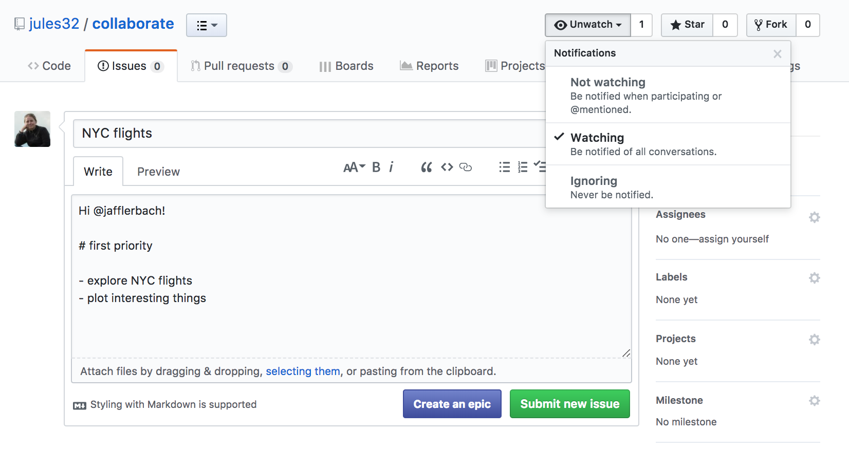
Let’s have Person 2 respond to the issue affirming the plan.
5.4 NYC flights exploration
Let’s continue this workflow with your collaborator, syncing to GitHub often and practicing what we’ve learned so far. We will get started together and then you and your collaborator will work on your own.
Here’s what we’ll be doing (from R for Data Science’s Transform Chapter):
Data: You will be exploring a dataset on flights departing New York City in 2013. These data are actually in a package called nycflights13, so we can load them the way we would any other package.
Let’s have Person 1 write this in the RMarkdown document (Partner 2 just listen for a moment; we will sync this to you in a moment).
library(nycflights13) # install.packages('nycflights13')
library(tidyverse)
This data frame contains all flights that departed from New York City in 2013. The data comes from the US Bureau of Transportation Statistics, and is documented in ?flights.
flights
Let’s select all flights on January 1st with:
filter(flights, month == 1, day == 1)
To use filtering effectively, you have to know how to select the observations that you want using the comparison operators. R provides the standard suite: >, >=, <, <=, != (not equal), and == (equal). We learned these operations yesterday. But there are a few others to learn as well.
Sync
Sync this RMarkdown back to GitHub so that your collaborator has access to all these notes.
Partner 2 pull
Now is the time to pull.
Partner 2 will continue with the following notes and instructions:
Logical operators
Multiple arguments to filter() are combined with “and”: every expression must be true in order for a row to be included in the output. For other types of combinations, you’ll need to use Boolean operators yourself:
&is “and”|is “or”!is “not”
Let’s have a look:
The following code finds all flights that departed in November or December:
filter(flights, month == 11 | month == 12)
The order of operations doesn’t work like English. You can’t write filter(flights, month == 11 | 12), which you might literally translate into “finds all flights that departed in November or December”. Instead it finds all months that equal 11 | 12, an expression that evaluates to TRUE. In a numeric context (like here), TRUE becomes one, so this finds all flights in January, not November or December. This is quite confusing!
A useful short-hand for this problem is x %in% y. This will select every row where x is one of the values in y. We could use it to rewrite the code above:
nov_dec <- filter(flights, month %in% c(11, 12))
Sometimes you can simplify complicated subsetting by remembering De Morgan’s law: !(x & y) is the same as !x | !y, and !(x | y) is the same as !x & !y. For example, if you wanted to find flights that weren’t delayed (on arrival or departure) by more than two hours, you could use either of the following two filters:
filter(flights, !(arr_delay > 120 | dep_delay > 120))
filter(flights, arr_delay <= 120, dep_delay <= 120)
Whenever you start using complicated, multipart expressions in filter(), consider making them explicit variables instead. That makes it much easier to check your work.
Partner 2 sync
Once you have filtered the flights dataframe for flights, sync it to Github (add, commit and push).
Your turn
Based on what you’ve learned previously about data transformation, you’ll make a series of data transformation on the flights dataset. Some ideas:
- calculate the average flight delay.
- determine the longest flight distance.
- Your own question!
Exercise
Partner 1 will pull so that we all have the most current information. With your partner, transform and compute several metrics about the data. Partner 1 and 2, make sure you talk to each other and decide on who does what. Remember to make your commit messages useful! As you work, you may get merge conflicts. This is part of collaborating in GitHub; we will walk through and help you with these and also teach the whole group.
6. Resources and credits
6.1 Useful links
- Creating a GitHub organization for a research lab
- Connecting a local
gitfolder to an existing GitHub remote
6.2 Icons
Key Points
Github allows you to synchronise work efforts and collaborate with other scientists on (R) code.
Github can be used to make custom website visible on the internet.
Merge conflicts can arise between you and yourself (different machines).
Merge conflicts arise when you collaborate and are a safe way to handle discordance.
Efficient collaboration on data analysis can be made using Github.
Become a champion of open (data) science
Overview
Teaching: 30 min
Exercises: 60 minQuestions
Objectives
To understand the importance to share data and code
To value code and data for what they are: the true foundations of any scientific statement.
To promote good practices for open & reproducible science
The Crisis of Confidence
The crisis of confidence poses a general problem across most empirical research disciplines and is characterized by an alarmingly low rate of key findings that are reproducible (e.g., Fidler et al. 2017; Open Science Collaboration, 2015; Poldrack et al., 2017; Wager et at., 2009). A low reproducibility rate can arise when scientists do not respect the empirical cycle. Scientific research methods for experimental research are based on the hypothetico-deductive approach (see e.g., de Groot, 1969; Peirce, 1878), which is illustrated in Figure 1.
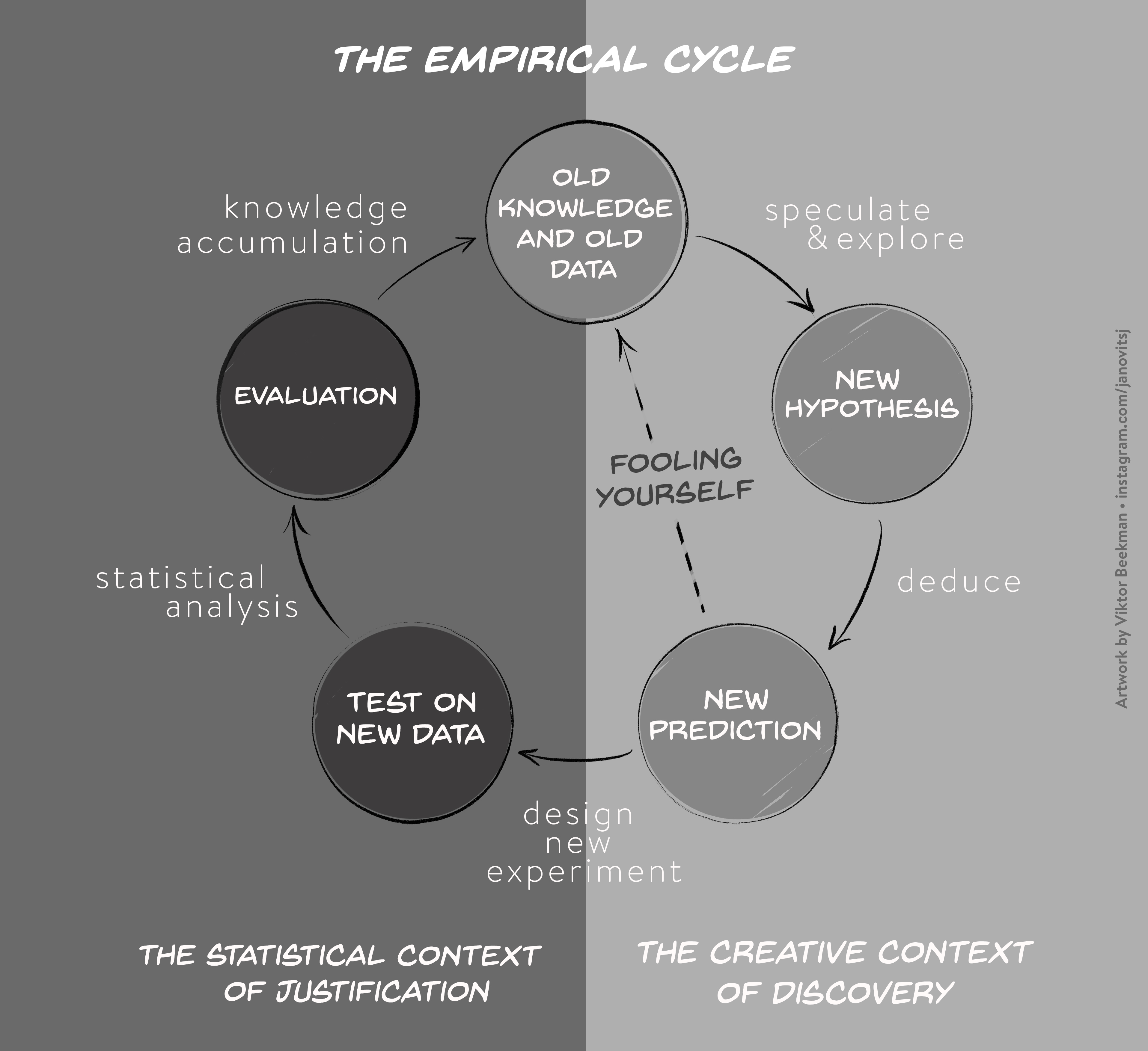
The empirical cycle suggests that scientists initially find themselves in “the creative context of discovery”, where the primary goal is to generate hypotheses and predictions based on exploration and data-dependent analyses. Subsequently, this initial stage of discovery is followed by “the statistical context of justification”. This is the stage of hypothesis-testing in which the statistical analysis must be independent of the outcome. Scientists may fool themselves whenever the results from the creative context of discovery with its data-dependent analyses are treated as if they came from the statistical context of justification. Since the selection of hypotheses now capitalizes on chance fluctuations, the corresponding findings are unlikely to replicate.
This suggests that the crisis of confidence is partly due to a blurred distinction between statistical analyses that are pre-planned and post-hoc, caused by the scientists degree of freedom in conducting the experiment, analyzing the data, and reporting the outcome. In a research environment with a high degree of freedom it is tempting to present the data exploration efforts as confirmatory (Carp, 2013). Kerr (1998, p. 204) attributed this biased reporting of favorable outcomes to an implicit effect of a hindsight bias: “After we have the results in hand and with the benefit of hindsight, it may be easy to misrecall that we had really ‘known it all along’, that what turned out to be the best post hoc explanation had also been our preferred a priori explanation.”
To overcome the crisis of confidence the research community must change the way scientists conduct their research. The alternatives to current research practices generally aim to increase transparency, openness, and reproducibility. Applied to the field of ecology, Ellison (2010, p. 2536) suggests that “repeatability and reproducibility of ecological synthesis requires full disclosure not only of hypotheses and predictions, but also of the raw data, methods used to produce derived data sets, choices made as to which data or data sets were included in, and which were excluded from, the derived data sets, and tools and techniques used to analyze the derived data sets.” To facilitate their uptake, however, it is essential that these open and reproducible research practices are concrete and practical.
Open and Reproducible Research Practices
In this section, we focus on open and reproducible research practices that researchers can implement directly into their workflow, such as data sharing, creating reproducible analyses, and the preregistration of studies.
Data Sharing
International collaboration is a cornerstone for the field of ecology and thus the documentation, and archiving of large volume of (multinational) data and metadata is becoming increasingly important. Even though many scientists are reluctant to make their data publicly available, data sharing can increase the impact of their research. For instance, in cancer research, studies for which data were publicly available received higher citation rates compared to studies for which data were not available (Piwowar, Day, & Fridsma, 2007). This is due to the fact that other researchers can build directly on existing data, analyze them using utilize novel statistical techniques and modelling tools, and mine them from new perspectives (Carpenter et al., 2009).
Reproducibility of Statistical Results
One of the core scientific values is reprodicibility. The reproducibility of experimental designs and methods allows the scientific community to determine the validity of alledged effects.
The benefit of publishing fully reporducible statistical results (including the reporting of all data preprocessing steps) is that collaborators, peer-reviewers, and independent researchers can repeat the analysis –from raw data and to the creation of relevant figures and tables– and verify the correctness of the results. Scientific articles are not free from typographical mistakes and it has been shown that the prevalence for statistical reporting errors is shockingly high. For instance, Nuijten et al. (2015) examined the prevalence of statistical reporting errors in the field of psychology and found that almost 50% or all psychological articles papers contain at least one error. These reporting errors can lead to erroneous substantive conclusions and influence, for instance, the results of meta-analyses. Most importantly, however, is that these errors are preventable. Through tools, such as git and RMarkdown, researchers can automate their statistical reporting and produce fully reproducible research papers.
Preregistration and Registered Reports
A blurred distinction between statistical analyses that are pre-planned and post-hoc causes many researchers to (unintentionally) use questionable research practices to produce significant findings (QRPs; John, Loewenstein, & Prelec, 2012). The most effective method to combat questionable research practices is preregistration, a procedure to curtail scientists’ degrees of freedom (e.g., Wagenmakers & Dutilh, 2016. When preregistering studies, scientists commit to an analysis plan in advance of data collection. By making a sharp distinction between hypothesis generating and analyzing the data, preregistration eliminates the confusion between exploratory and confirmatory research.
Over the last years, preregistration has quickly gained popularity and has established itself over several platforms and formats. Scientists can now choose to preregister their work either independently —for instance on platforms like https://asPredicted.org or the Open Science Framework (OSF)— or preregister their studies directly in a journal in the format of a Registered Report as promoted by Chris Chambers (2013). Currently about 200 journals —including Nature: Human Behaviour— accept Registered Reports either as a regular submission option or as part of a single special issue (see https://cos.io/rr/ for the full list).
Preregistration is encouraged in the transparency and openness promotion (TOP) guidelines (Nosek et al., 2015 and represents the standard for the analysis of clinical trials; for instance, in the New England Journal of Medicine —the world’s highest impact journal— the registration of Clinical Trials is a prerequisite for publication.
Challenges
- Data sharing: ethical concerns (share data that harm others, e.g., lowering property values or private data that are collected, for instance, through satellites); Solution = share anonimized data, policies need to be developed
- Preregistration: Loosing the flexibility to adapt analysis plans to unexpected peculiarities of the data; Solution = data blinding, which is standard practice in astrophysics)
- Reproducibility: Additional costs associated with the time it takes to adequatly annotate and archive the code so that independent researchers can understand and reproduce fugures and results; Solution = reproducible workflow, for instance by working in Git and Rmarkdown
Potential Exercises on this Topic
Ideas for exercises are taken from Sarafoglou, A., Hoogeveen, S., Matzke, D., & Wagenmakers, E.-J. (2019). Teaching Good Research Practices: Protocol of a Research Master Course. Psychology Learning & Teaching. This article describes the full course catalogue of the Research Master course ‘Good Research Practices’ which is taught at the University of Amsterdam. The description of in-class assignments can be found here: https://osf.io/5xjfh/
Potential in-class assignments are:
- Ivestigate the Transparency of Empirical Articles: https://osf.io/p7xtj/
- Hidden Flexibility in Data Analysis: https://osf.io/y4h25/
Three messages
If there are 3 things to communicate to others after this workshop, I think they would be:
1. Data science is a discipline that can improve your analyses
- There are concepts, theory, and tools for thinking about and working with data.
- Your study system is not unique when it comes to data, and accepting this will speed up your analyses.
This helps your science:
- Think deliberately about data: when you distinguish data questions from research questions, you’ll learn how and who to ask for help
- Save heartache: you don’t have to reinvent the wheel
- Save time: when you expect there’s a better way to do what you are doing, you’ll find the solution faster. Focus on the science.
2. Open data science tools exist
- Data science tools that enable open science are game-changing for analysis, collaboration and communication.
- Open science is “the concept of transparency at all stages of the research process, coupled with free and open access to data, code, and papers” (Hampton et al. 2015)
- For empirical researchers: transparency checklist (https://eltedecisionlab.shinyapps.io/TransparencyChecklist/)
- Repositories such as the Open Science Framework (https://osf.io/preregistration) offer preregistration templates and the tools to archive your projects
This helps your science:
- Blogpost: Seven Reasons To Work Reproducibly (written by the Center of Open Science): https://cos.io/blog/seven-reasons-work-reproducibly/
- Have confidence in your analyses from this traceable, reusable record
- Save time through automation, thinking ahead of your immediate task, reduced bookkeeping, and collaboration
- Take advantage of convenient access: working openly online is like having an extended memory _ Making your data and code publicly available can increase the impact of research.
3. Learn these tools with collaborators and community (redefined):
- Your most important collaborator is Future You.
- Community should also be beyond the colleagues in your field.
- Learn from, with, and for others.
This helps your science:
- If you learn to talk about your data, you’ll find solutions faster.
- Build confidence: these skills are transferable beyond your science.
- Be empathetic and inclusive and build a network of allies
Build and/or join a local coding community
Join existing communities locally and online, and start local chapters with friends!
Some ideas:
-
Amsterdam Science Park Study Group Slack workspace: join this workspace to ask questions and network with other biologists on programming and data analysis topics. Slack is a collaboration software used mostly by companies that has more than 10 million users worldwide.
-
Amsterdam Science Park Study Group: this local Mozilla Study Groups is regularly organising local training workshops for biologists that are either beginners or more advanced in scientific programming. A publication describing the intention of these study groups and how to implement them has been published in 2018 in PLoS Biology.
-
RLadies. Informal but efficient communities centered on R data analysis meant to be inclusive and supportive. The RLadies Amsterdam chapter is quite active in Amsterdam!
These meetups can be for skill-sharing, showcasing how people work, or building community so you can troubleshoot together. They can be an informal “hacky hour” at a cafe or pub!
Going further / Bibliography
- The Replication Crisis in Wikipedia
- A special issue in Science on Reproducibility
- Open Science And Reproducibility: presentation by Alexandra Sarafoglou (PhD student, UvA)
Key Points
Make your data and code available to others
Make your analyses reproducible
Make a sharp distincion between exploratory and confirmatory research